brain of mat kelcey...

neural nets on the daisy patch?

the electro smith daisy patch is a eurorack module made for prototyping; it provides a powerful audio focussed microcontroller setup (the daisy 'seed' with arm cortex-m7 running at 480MHz) along with all the connectivity required to be a eurorack module.

pretty much the first thing i thought when i saw one was; "could it run a neural net?" microcontrollers are fast, but so too is audio rate.

note: see also the updated version of this project running on an FPGA though it's worth reading this first to understand the model and waveshaping task

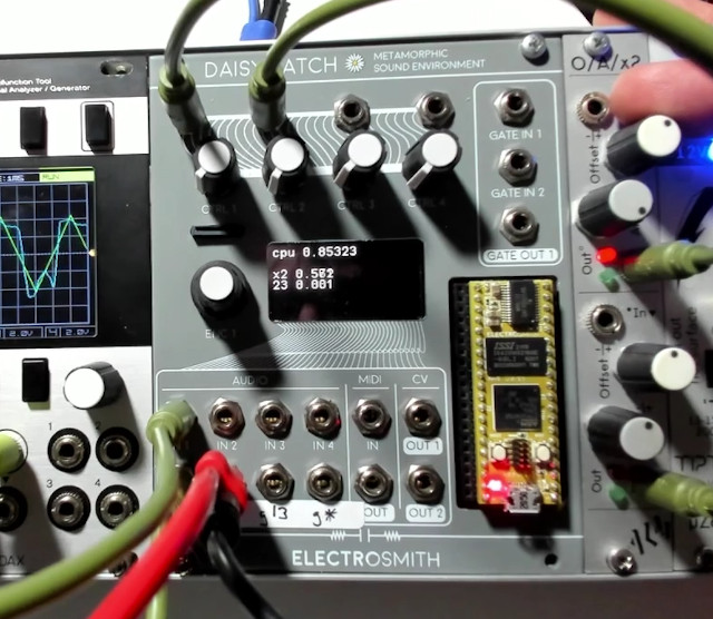
after a bit of research i found there are a couple of people who have done some real time audio effects processing on the daisy seed; e.g. guitarML's neural seed

all the examples i found though were quite small recurrent models and i was keen to give wavenet a go instead ( i'm a big fan of causal dilated convolutions )

wavenet 101

the wavenet architecture is a 1D convolutional network designed to operate on timeseries data. it is composed of two key structures;

• it uses causal padding to ensure that each convolution never depends on anything from the future and
• it increases dilation exponentially each layer to give the following structure

usually it's just dilation convolutions stacked but for my variant i also include one extra 1x1 conv between each dilation; a 1x1 doesn't break any of the dilation structure wavenet needs and including another non linearity is almost always a good thing.

training

the first step was to write a firmware that just recorded some audio and/or control voltages into buffers and then streamed them out over a serial connection. it's kinda clumsy, and i'm sure there's a cleaner way, but it works without having to mess around too much. the code is datalogger_firmware/

from there a wavenet could be trained ( see keras_model.py ) and it was trivial to quantise and export to a c++ lib for the microcontroller using edge impulse's bring-your-own-model

from there i got a bit stuck though integrating tensorflow with the daisy optimised arm_math.h stuff ( Make files and such aren't my expertise ) so instead i thought i'd use this chance to write my own inference. convolutions don't need much, it's all just a bunch of matrix math after all.

while poking around doing this it suddenly occured to me that you could do heavy heavy caching of the convolution activations! i was super excited, thinking i was doing some novel, and it wasn't until i was actually finished that i found out someone else had thought of the same idea basically, what they call fast-wavenet :/

oh well, it was fun to discover independently i suppose, and i ended up implementing things a bit differently.

caching activations for inference

so let's walk through the caching optimisation...

consider the following wavenet like network; it has 16 inputs being integrated thru 3 layers to a single prediction

if we consider a sliding window input at time step 4 we see that the output of node 0 ( the node with the red 0 ) will be the processed values from [0, 1, 2, 3]

a bit later on an interesting things happens at time step 8; node 1 now gets the same inputs that node 0 had 4 steps ago.

so we don't need to calculate it! when processing a timeseries we can see that the node 1 output just lags node 0 by 4 steps, and nodes 2 and 3 lag another 4 each. as long as we've got the memory for caching we can store all these in a circular buffer.

and this whole thing is stackable! in fact we only ever need to run the right hand side convolutions, as long as we have the memory to cache.

one big win for this on the daisy is that it can all run fast and small enough that we can use full float32 math everywhere. hoorah!

in terms of coding the whole thing becomes an exercise in

1. preparing the data in the right way to pass to some crazy optimised linear algebra math and
2. doing so with as little memory copying as possible :/

representative architectures

the following model has an input of 3 values => a receptive field of 256 steps, and a single output. it runs on the daisy using the above caching technique at 48KHz @88% CPU ( ~20 micro seconds per inference ). we'll describe what the 3 input values are in a bit. it's the model we'll use the examples at the end.

cNa - denotes the dilated convolutions
cNb - denotes the 1x1s convolutions that follow cNa
F - number of filters
K - kernel size; either 4 for cNa or 1 for cNb
D - dilation; K^layer# for cNa, or 1 for cNb
P - padding; 'causal' or the layer dft 'valid'

____________________________________________________________________________________________
 Layer (type)         Output Shape      Par#  Conv1D params   
============================================================================================
 input (InputLayer)   [(None, 256, 3)]  0                                   
 c0a (Conv1D)         (None, 64, 4)     52    F=4, K=4, D=1, P=causal
 c0b (Conv1D)         (None, 64, 4)     20    F=4, K=1
 c1a (Conv1D)         (None, 16, 4)     68    F=4, K=4, D=4, P=causal
 c1b (Conv1D)         (None, 16, 4)     20    F=4, K=1
 c2a (Conv1D)         (None, 4, 4)      68    F=4, K=4, D=16, P=causal
 c2b (Conv1D)         (None, 4, 4)      20    F=4, K=1
 c3a (Conv1D)         (None, 1, 8)      136   F=8, K=4, D=64, P=causal        
 c3b (Conv1D)         (None, 1, 8)      72    F=8, K=1
 y_pred (Conv1D)      (None, 1, 1)      13    F=1, K=1
============================================================================================
Total params: 465
____________________________________________________________________________________________

as a side note, the daisy can actually run at 96kHz but at this rate i could only run a smaller [c0a, c0b, c1a, c2b] model with just 2 filters each. it runs, but i couldn't get it to train on the examples i show below, so i didn't use it. shame because naming the blog post "at (almost) 100,000 inferences a second" would have had a nicer ring to it :D

it can also run slower, e.g. 32kHz, which allows either more filters per step, or even more depth => large receptive field.

but these combos demonstrate an interesting set of trade offs we have between

• depth ( which dictates the receptive field / input size )
• number of filters we can manage and
• what audio rate we can run at.

for training i just use keras.layer.Conv1D everywhere but then exported to the device in two passes; a python prototype and then the c++ code for the device.

cmsis-dsp

the final code on the daisy uses the cmsis-dsp library for all the matrix math. only three pieces end up being used though

• arm_mat_init_f32 for making the matrix structures,
• arm_mat_mult_f32 for the actual matrix multiplications and
• arm_add_f32 for the kernel accumulation and adding biases here and there.

to be honest none of these were benchmarked and i assume they are faster than if the multiplications were just rolled out (???)

python cmsis-dsp prototype

the first pass was to get the inference working as a prototype in python. the cmsisdsp python lib was used ( a pure python api equivalent ) and the code is cmsisdsp_py_version/.

having cmsisdsp was very handy to prototype, especially as i've not done any cmsis stuff before.

cmsis on the daisy

the code for the daisy is under inference_firmware/ and is a port of the python version. it's where i probably spent the most amount of time, especially block.h

it has 4 main parts

• left_shift_buffer.h to handle the shifted InputLayer
• block.h to handle the sequential running of each cNa and cNb pair
• rolling_cache.h which represents the circular buffer used for activation lag and
• regression.h which is just a simple y=mx+b using the weights from the final 1x1 Conv1D regression used during training

it all ends up being pretty straightforward but i did iterate a bit; any code involving memcpy and pointer arithmetic needs careful attention.

the "best" bit of the code is where the initial kera model is trained in a python notebook and then exported to be used in the c++ code by having python code construct a model_defn.h with a bunch of print statements :/ it's actually written to /tmp/model_defn.h no less! what a hack, lol. may god have mercy on my soul.

an example waveshaper

for a demo project i wanted to make a little waveshaper; something that takes one waveform and outputs another.

so 5 waveforms were collected from another eurorack oscillator; a triangle, sine, saw, square and a weird zigzag thing. during data collection random voltages were sampled to change the oscillator's frequency.

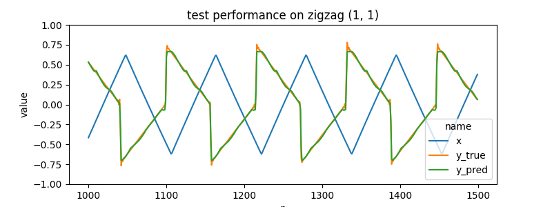
to convert to actual training dataset the triangle wave is used as input with one of the other waves acting as output. which output is decided by including two additional selector variables in the inputs. these variables are only ever {0, 1} during training but can act (very loosely) as an embedding since any float value can be passed in the range (0, 1) when running on the device.

input	output
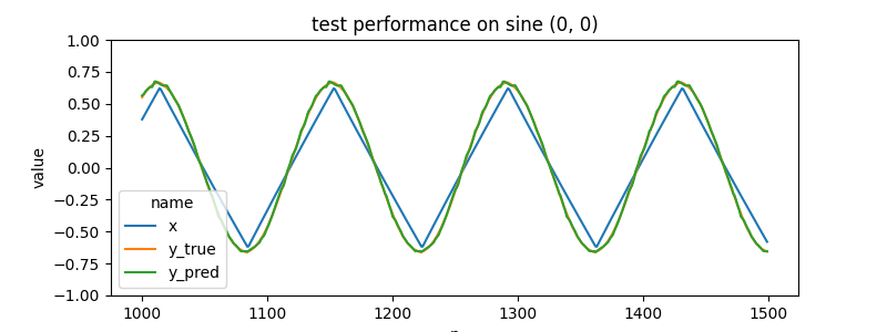
(triangle, 0, 0)	sine
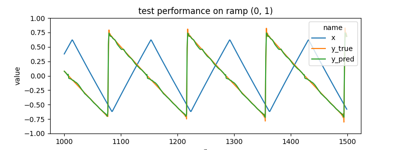
(triangle, 0, 1)	ramp
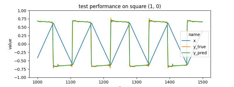
(triangle, 1, 0)	square
(triangle, 1, 1)	zigzag

the model was trained for < 1 min ( the model is pretty small, and there's not much variety in the data ).

it does well on held out test data...

but the much more interesting thing is what happens when we input values for x2 and x3 that weren't see during training data

e.g. what if we choose a point that is 20% between sine (0, 0) and square (1, 0) ? we end up with some weird non defined part of the input space.

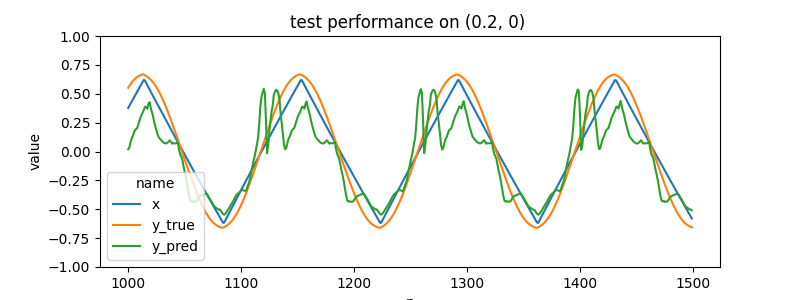these out of training distribution things are always the most interesting to me; values for x2 and x3 inbetween (0, 1) give a weird sort-of-interpolation. generally these results are never a smooth transistion unless there's some aspect of the loss that directs it to be so (and in this case there isn't).

we get the classic model hallucination stuff that i've always loved. ( see my older post on hallucinating softmaxs for more info )

we could encourage the model to make full use of the space by including a GAN like discriminator loss. this would be trained on random samples of values for (x2, x3). i've seen this kind of training force the model to be much more consistent for interpolated inputs.

this video of the network actually running give a better idea of the "interpolation". the green wave shows the input core triangle wave, the blue wave shows the output waveshaped result. the daisy module display shows the values for x2 and x3; with these values controlled by hand from the module on the right.

the video transistions across values of (x2, x3), moving between the corner (0, 1) values. at each corner the frequency of the core triangle input wave was adjusted over a range as well. something i hadn't considered is that when we change the frequency to be outside the range of what was seen during training the model does some weird extrapolation.

the interpolation extrapolation stuff makes some weird things, but it all sounds cool :)

appendix

further ideas could be...

• use mulaw encoding? the originl deepmind wavenet paper talks about the model output being a distribution across mulaw encoded values. that's interesting; i've used mulaw for compression in loopers and delays, but never as a categorical thing to classify!
• there's other things we can add in the block; e.g. is this model too small to use a skip connection around the 1x1 block?
• further study on relationship of audio rate vs dilation/receptive field
• GAN discriminator across randomly sampled (x2, x3)
• this is all running in float32 math but there's a number of quantised operators available too. how much bigger/faster could the network be if we swap toi quantised calculations?

note: see also the updated version of this project running on an FPGA

code on github