embedding lookup tables

one thing in theano i couldn't immediately find examples for was a simple embedding lookup table, a critical component for anything with NLP. turns out that it's just one of those things that's so simple no one bothered writing it down :/

tl;dr : you can just use numpy indexing and everything just works.

numpy / theano indexing

consider the following theano.tensor example of 2d embeddings for 5 items. each row represents a seperate embeddable item.

>>> E = np.random.randn(5, 2)
>>> t_E = theano.shared(E)
>>> t_E.eval()
array([[-0.72310919, -1.81050727],
       [ 0.2272197 , -1.23468159],
       [-0.59782901, -1.20510837],
       [-0.55842279, -1.57878187],
       [ 0.63385967, -0.35352725]])

to pick a subset of the embeddings it's as simple as just using indexing. for example to get the third & first embeddings it's ...

>>> idxs = np.asarray([2, 0])
>>> t_E[idxs].eval()
array([[-0.59782901, -1.20510837],   # third row of E
       [-0.72310919, -1.81050727]])  # first row of E

if we want to concatenate them into a single vector (a common operation when we're feeding up to, say, a densely connected hidden layer), it's a reshape

>>> t_E[idxs].reshape((1, -1)).eval()
array([[-0.59782901, -1.20510837, -0.72310919, -1.81050727]])  # third & first row concatenated

all the required multi dimensional operations you need for batching just work too..

eg. if we wanted to run a batch of size 2 with the first batch item being the third & first embeddings and the second batch item being the fourth & fourth embeddings we'd do the following...

>>> idxs = np.asarray([[2, 0], [3, 3]])  # batch of size 2, first example in batch is pair [2, 0], second example in batch is [3, 3]
>>> t_E[idxs].eval()
array([[[-0.59782901, -1.20510837],    # third row of E
        [-0.72310919, -1.81050727]],   # first row of E
       [[-0.55842279, -1.57878187],    # fourth row of E
        [-0.55842279, -1.57878187]]])  # fourth row of E
>>> t_E[idxs].reshape((idxs.shape[0], -1)).eval()
array([[-0.59782901, -1.20510837, -0.72310919, -1.81050727],   # first item in batch; third & first row concatenated
       [-0.55842279, -1.57878187, -0.55842279, -1.57878187]])  # second item in batch; fourth row duplicated

this type of packing of the data into matrices is crucial to enable linear algebra libs and GPUs to really fire up.

a trivial full end to end example

consider the following as-simple-as-i-can-think-up "network" that uses embeddings;

given 6 items we want to train 2d embeddings such that the first two items have the same embeddings, the third and fourth have the same embeddings and the last two have the same embeddings. additionally we want all other combos to have different embeddings.

the entire theano code (sans imports) is the following..

first we initialise the embedding matrix as before

E = np.asarray(np.random.randn(6, 2), dtype='float32')
t_E = theano.shared(E)

the "network" is just a dot product of two embeddings ...

t_idxs = T.ivector()
t_embedding_output = t_E[t_idxs]
t_dot_product = T.dot(t_embedding_output[0], t_embedding_output[1])

... where the training cost is a an L1 penality against the "label" of 1.0 for the pairs we want to have the same embeddings and 0.0 for the ones we want to have a different embeddings.

t_label = T.iscalar()
gradient = T.grad(cost=abs(t_label - t_dot_product), wrt=t_E)
updates = [(t_E, t_E - 0.01 * gradient)]
train = theano.function(inputs=[t_idxs, t_label], outputs=[], updates=updates)

we can generate training examples by randomly picking two elements and assigning label 1.0 for the pairs 0 & 1, 2 & 3 and 4 & 6 (and 0.0 otherwise) and every once in awhile write them out to a file.

print "i n d0 d1"
for i in range(0, 10000):
    v1, v2 = random.randint(0, 5), random.randint(0, 5)
    label = 1.0 if (v1/2 == v2/2) else 0.0
    train([v1, v2], label)
    if i % 100 == 0:
        for n, embedding in enumerate(t_E.get_value()):
            print i, n, embedding[0], embedding[1]

plotting this shows the convergence of the embeddings (labels denote initial embedding location)...

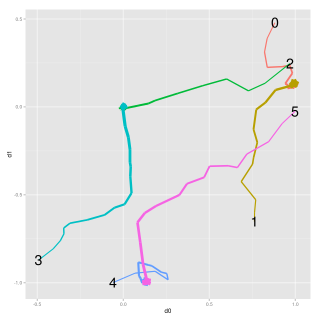
0 & 1 come together, as do 2 & 3 and 4 & 5. ta da!

a note on dot products

it's interesting to observe the effect of this (somewhat) arbitrary cost function i picked.

for the pairs where we wanted the embeddings to be same the cost function, \( |1 - a \cdot b | \), is minimised when the dotproduct is 1 and this happens when the vectors are the same and have unit length. you can see this is case for pairs 0 & 1 and 4 & 5 which have come together and ended up on the unit circle. but what about 2 & 3? they've gone to the origin and the dotproduct of the origin with itself is 0, so it's maximising the cost, not minimising it! why?

it's because of the other constraint we added. for all the pairs we wanted the embeddings to be different the cost function, \( |0 - a \cdot b | \), is minimised when the dotproduct is 0. this happens when the vectors are orthogonal. both 0 & 1 and 4 & 5 can be on the unit sphere and orthogonal but for them to be both orthogonal to 2 & 3 they have to be at the origin. since my loss is an L1 loss (instead of, say, a L2 squared loss) the pair 2 & 3 is overall better at the origin because it gets more from minimising this constraint than worrying about the first.

the pair 2 & 3 has come together not because we were training embeddings to be the same but because we were also training them to be different. this wouldn't be a problem if we were using 3d embeddings since they could all be both on the unit sphere and orthogonal at the same time.

you can also see how the points never fully converge. in 2d with this loss it's impossible to get the cost down to 0 so they continue to get bumped around. in 3d, as just mentioned, the cost can be 0 and the points would converge.

a note on inc_subtensor optimisation

there's one non trivial optimisation you can do regarding your embeddings that relates to how sparse the embedding update is. in the above example we have 6 embeddings in total and, even though we only update 2 of them at a time, we are calculating the gradient with respect to the entire t_E matrix. the end result is that we calculate (and apply) a gradient that for the majority of rows is just zeros.

...
gradient = T.grad(cost=abs(t_label - t_dot_product), wrt=t_E)
updates = [(t_E, t_E - 0.01 * gradient)]
...
print gradient.eval({t_idxs: [1, 2], t_label: 0})
[[  0.00000000e+00   0.00000000e+00]
 [  9.60363150e-01   2.22545816e-04]
 [  1.00614786e+00  -3.63630615e-03]
 [  0.00000000e+00   0.00000000e+00]
 [  0.00000000e+00   0.00000000e+00]
 [  0.00000000e+00   0.00000000e+00]]

you can imagine how much sparser things are when you've got 1M embeddings and are only updating <10 per example :/

rather than do all this wasted work we can be a bit more explicit about both how we want the gradient calculated and updated by using inc_subtensor

...
t_embedding_output = t_E[t_idxs]
...
gradient = T.grad(cost=abs(t_label - t_dot_product), wrt=t_embedding_output)
updates = [(t_E, T.inc_subtensor(t_embedding_output, -0.01 * gradient))]
...
print gradient.eval({t_idxs: [1, 2], t_label: 0})
[[  9.60363150e-01   2.22545816e-04]
 [  1.00614786e+00  -3.63630615e-03]]

and of course you should only do this once you've proven it's the slow part...

for code, see this gist