


brain of mat kelcey...
differentiable kalman filters in jax
March 29, 2024 at 06:45 PM | categories: jaxkalman filters
was doing some work with kalman filters recently and, as always, wasn't sure what the best way to tune the filter configuration.
in the past i've taken a simple grid/random search like approach but was curious how i could express this tuning as an optimisation using jax instead.
first though, what is a kalman filter? they are pretty broad concept but the main thing i've used them for is dynamic system prediction.
they operate in a two step fashion...
- a
predictstep which predicts something about the system based on some internal state and - an
updatestep which integrates new observation information into the filter's state ready for the nextpredict
in this post we'll use a simple 2D trajectory as the system. e.g. throwing an object
the task of the kalman filter to be the prediction of the objects' position at the next time step
a simple dynamics system
consider then the simple system of throwing an object under a trivial physics model
def simulate_throw(dx, dy):
  x, y = 0, 0
  for _ in range(10):
    yield x, y
    x += dx
    y += dy
    dy -= 1
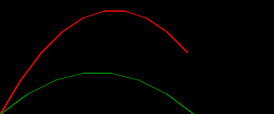
we can use this to simulate a couple of throws and plot the trajectories...
draw_throw_with_colours(
    [simulate_throw_a(dx=3, dy=5), simulate_throw_a(dx=4, dy=3)],
    ['red', 'green']
)
a numpy kalman filter implementation
can we use a kalman filter to predict the next state of these systems? i do hope so, it's what they were designed for!
implementations of a kalman filter can vary a lot so let's just use this random kalman filter from the internet
note: using this implementation, on any random snippet of code from the internet, for, say, controlling a rocket or something might be correctly considered a generally "bad idea". the correctness, or otherwise, of this filter is irrelevant to the task of jaxifying it :)
# as is from https://machinelearningspace.com/2d-object-tracking-using-kalman-filter/ with some
# minor changes

class KalmanFilter(object):
  def __init__(self, dt, u_x,u_y, std_acc, x_std_meas, y_std_meas):
    """
    :param dt: sampling time (time for 1 cycle)
    :param u_x: acceleration in x-direction
    :param u_y: acceleration in y-direction
    :param std_acc: process noise magnitude
    :param x_std_meas: standard deviation of the measurement in x-direction
    :param y_std_meas: standard deviation of the measurement in y-direction
    """
    # Define sampling time
    self.dt = dt
    # Define the  control input variables
    self.u = np.matrix([[u_x],[u_y]])
    # Intial State
    self.x = np.matrix([[0, 0], [0, 0], [0, 0], [0, 0]])
    # Define the State Transition Matrix A
    self.A = np.matrix([[1, 0, self.dt, 0],
                        [0, 1, 0, self.dt],
                        [0, 0, 1, 0],
                        [0, 0, 0, 1]])
    # Define the Control Input Matrix B
    self.B = np.matrix([[(self.dt**2)/2, 0],
                        [0, (self.dt**2)/2],
                        [self.dt, 0],
                        [0, self.dt]])
    # Define Measurement Mapping Matrix
    self.H = np.matrix([[1, 0, 0, 0],
                        [0, 1, 0, 0]])
    # Initial Process Noise Covariance
    self.Q = np.matrix([[(self.dt**4)/4, 0, (self.dt**3)/2, 0],
                        [0, (self.dt**4)/4, 0, (self.dt**3)/2],
                        [(self.dt**3)/2, 0, self.dt**2, 0],
                        [0, (self.dt**3)/2, 0, self.dt**2]]) * std_acc**2
    # Initial Measurement Noise Covariance
    self.R = np.matrix([[x_std_meas**2,0],
                        [0, y_std_meas**2]])
    # Initial Covariance Matrix
    self.P = np.eye(self.A.shape[1])

  def predict(self):
    # Refer to :Eq.(9) and Eq.(10)
    # Update time state
    #x_k =Ax_(k-1) + Bu_(k-1)     Eq.(9)
    self.x = np.dot(self.A, self.x) + np.dot(self.B, self.u)
    # Calculate error covariance
    # P= A*P*A' + Q               Eq.(10)
    self.P = np.dot(np.dot(self.A, self.P), self.A.T) + self.Q
    return self.x[0]

  def update(self, z):
    # Refer to :Eq.(11), Eq.(12) and Eq.(13)
    # S = H*P*H'+R
    S = np.dot(self.H, np.dot(self.P, self.H.T)) + self.R
    # Calculate the Kalman Gain
    # K = P * H'* inv(H*P*H'+R)
    K = np.dot(np.dot(self.P, self.H.T), np.linalg.inv(S))  #Eq.(11)
    self.x = self.x + np.dot(K, (z - np.dot(self.H, self.x)))   #Eq.(12)
    I = np.eye(self.H.shape[1])
    # Update error covariance matrix
    self.P = (I - (K * self.H)) * self.P   #Eq.(13)
a couple of things to note about this filter
- recall the api is two methods;
predictwhich provides an estimate ofxandupdatewhich updates the internal state of the filter based on a real observation. the implementations of these are kinda opaque and i wouldn't be surprised if there are a stack of subtle bugs here that a dynamic systems expert could spot. i am happy to take it "as is" for the purpose of poking around in some jax - since both
predictandupdatechange the internal state of the filter it's expected they are called in sequence;predict,update,predict,updateetc - there are a bunch of cryptically named variables;
u,B,Hetc, some of which are to do with the internal state of the filter ( likeP) with others representing a form of config around how we expect the dynamics of the system to behave ( likeA). these latter matrices are configured based off scalar values such asdtandx_std_meas.
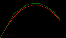
predicting a trajectory with the numpy kalman filter
we can use this filter as is to make predictions about the next time step of a throw, and it's not too bad at it...
# construct a filter with some config
filter = KalmanFilter(
    dt=1.0, u_x=0, u_y=0,
    std_acc=1.0, x_std_meas=0.1, y_std_meas=0.1)

# simulate a throw
xy_trues = simulate_throw(2.8, 4.8)

# step throw the trajectory
xy_preds = []
for xy_true in xy_trues:
  # make prediction based on filter and record it
  xy_pred = filter.predict()
  xy_preds.append(xy_pred)
  # update the filter state based on the true value
  filter.update(xy_true)

# plot the pair
# * red denotes true values,
# * green denotes predicted values based on the time step before
xy_preds = np.stack(xy_preds).squeeze()
draw_throw_with_colours(
    [xy_trues, xy_preds],
    ['red',    'green'])

porting to pure functional jax
next let's port this kalman filter to jax. there's a few aspects of this....
params and states
a key concept in the jax port is making predict and update fully functional,
and that means taking a state and returning it for the two methods. i.e. something like...
def predict(params, state):
  ...
  return state, xy_pred

def update(params, state, z):
  ...
  return state
we can then have all the P, A, Q, etc go in either params or state.
note: we are going to be explicit about two different types of variables we are dealing with here...
staterepresents the internal state of the filter that changes over time based on the sequence ofpredict,update,predict, ... callsparamsrepresents the configuration items, based ondtetc, that we eventually want to get gradients for ( with respect to a loss function )
the pairing of predict then update can be expressed as the following
that reassigns state each method call
def predict_then_update(params, state, xy_true):
  state, xy_pred = predict(params, state)
  state = update(params, state, xy_true)
  return state, xy_pred
what type are params and state then?
we want them to be collections of variables which are well supported in jax
under the idea of
pytrees
and we can get a lot way with just thinking of them as dictionaries...
note for this jax port:
- i switched from
jnp.dotto@which, IMHO, reads easier. - given no control inputs i've dropped
u_xandu_ywhich were 0.0s anyways. and nouimplies noBeither... - the implementation feels a bit clunky with dictionary look ups but oh well...
def predict(params, state):
  state['x'] = params['A'] @ state['x']
  state['P'] = ((params['A'] @ state['P']) @ params['A'].T) + params['Q']
  xy_pred = state['x'][0]
  return state, xy_pred

def update(params, state, z):
  # Define Measurement Mapping Matrix
  H = jnp.array([[1, 0, 0, 0],
                 [0, 1, 0, 0]])
  S = (H @ (state['P'] @ H.T)) + params['R']
  K = (state['P'] @ H.T) @ jnp.linalg.inv(S)
  state['x'] = state['x'] + (K @ (z - (H @ state['x'])))
  I = jnp.eye(4)
  state['P'] = (I - (K @ H)) @ state['P']
  return state
the final missing piece then is how we define the initial values for params and state
def default_params():
  dt = 1.0
  std_acc = 1.0
  x_std_meas, y_std_meas = 0.1, 0.1
  return {
    # Define the State Transition Matrix A
    'A': jnp.array([[1, 0, dt, 0],
                    [0, 1, 0, dt],
                    [0, 0, 1, 0],
                    [0, 0, 0, 1]]),
    # Initial Measurement Noise Covariance
    'R': jnp.array([[x_std_meas**2, 0],
                    [0, y_std_meas**2]]),
    # Initial Process Noise Covariance
    'Q': jnp.array([[(dt**4)/4, 0, (dt**3)/2, 0],
                    [0, (dt**4)/4, 0, (dt**3)/2],
                    [(dt**3)/2, 0, dt**2, 0],
                    [0, (dt**3)/2, 0, dt**2]]) * std_acc**2
  }

def initial_state():
  return {
    # Initial State
    'x': jnp.zeros((4, 2)),
    # Initial Covariance Matrix
    'P': jnp.eye(4),
  }
which all comes together like the numpy one as ...
params = default_params()
state = initial_state()
xy_trues = simulate_throw(2.8, 4.8)
xy_preds = []
for xy_true in xy_trues:
    state, xy_pred = predict_then_update(params, state, xy_true)
    xy_preds.append(xy_pred)
xy_preds = np.stack(xy_preds)

draw_throw_with_colours(
    [xy_trues, xy_preds],
    ['red',    'green'])
a minor diversion regarding rolling out kalman filters and teacher forcing.
before we go any deeper into jax land let's talk about one more aspect of using kalman filters.
the main idea touched on already is that we can use them to make a prediction about the next state of a system before we observe it.
xy_pred_t0 = predict()
# wait for actual xy_true_t0
update(xy_true_t0)
xy_pred_t1 = predict()
# wait for actual xy_true_t1
update(xy_true_t1)
but if we really trust the filter we can use it to alos handle missing observations by passing in the last predicted as the observed one when we don't have it ( for whatever reason )
xy_pred_t0 = predict()
# oh oh! for whatever reason we don't have _t0
update(xy_pred_t0)  # use predicted instead
xy_pred_t1 = predict()
# wait for actual xy_true_t1
update(xy_true_t1)
this can be handy for a signal that noisy and dropping out but it does put more pressure on the filter to be robust to any compounding error it might exhibit.
during training then ( which we still haven't talked about yet ) we can induce this
by occasionally randomly dropping out
xy_true values and using the prior xy_pred value instead.
( those with a background in RNNs might notice this is the same as teacher forcing )
the code to do this based on a 20% dropout can be....
def predict_then_update(params, state, has_observation, xy_true):
  state, xy_pred = predict(params, state)
  xy_for_update = jnp.where(has_observation, xy_true, xy_pred)
  state = update(params, state, xy_for_update)
  return state, xy_pred

xy_preds = []
has_observations = []
for xy_true in xy_trues:
  has_observation = rng.uniform() > 0.2
  has_observations.append(has_observation)
  state, xy_pred = predict_then_update(params, state, has_observation, xy_true)
  xy_preds.append(xy_pred)
xy_preds = np.stack(xy_preds)

print("has_observations", has_observations

draw_throw_with_colours(
    [xy_trues, xy_preds],
    ['red', 'green'])
has_observations [True, True, True, True, True, False, False, True, False, False]
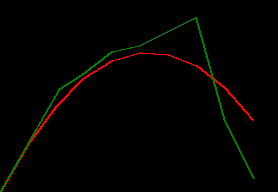
notice how the filter shoots way off after that pair of Falses. the default_params values
might be good enough to predict one step in the future, but they don't look robust to predicting two
or more steps in the future.
time to jax things up!!!
jax.lax.scan
a key first thing to do is to implement the for loop with jax.lax.scan so that jax can more cleanly trace it.
jax.lax.scan provides the classic functional programming idea of iterating over a method
with a carried state.
note:
- we move the random allocation of
has_observationinto the jax function which means having to assign akeyto thestatethat will be carried along between calls topredict_then_update_single - the scanning works cleanly because each
xy_truessequence is the same length. in the cases where we might have a different roll out length we'd need to use something like zero padding and loss masking or bucketing by sequence length. - we get the entire set of
xy_predsin a single call fromxy_trues
def initial_state(seed):
  return {
    # Initial State
    'x': jnp.zeros((4, 2)),
    # Initial Covariance Matrix
    'P': jnp.eye(4),
    # rng key for missing observations
    'key': jax.random.key(seed)
  }

def rolled_out_predict_then_update(params, seed, xy_trues, missing_rate):

  def predict_then_update_single(state, xy_true):
    state, xy_pred = predict(params, state)

    state['key'], subkey = jax.random.split(state['key'])
    has_observation = jax.random.uniform(subkey) > missing_rate
    xy_for_update = jnp.where(has_observation, xy_true, xy_pred)

    state = update(params, state, xy_for_update)
    return state, xy_pred

  _final_state, predictions = jax.lax.scan(predict_then_update_single, initial_state(seed), xy_trues)
  return predictions

xy_trues = np.array(list(simulate_throw(2.8, 4.8)))

seed = 1234414
xy_preds = jax.jit(rolled_out_predict_then_update)(default_params(), seed, xy_trues, missing_rate=0.2)

draw_throw_with_colours(
    [xy_trues, xy_preds],
    ['red',    'green'])
this example has a bunch of missed observations and the filter struggles quite a bit :/
a loss function, jax.grad & a simple training loop
with a function now that takes a list of xy_true values and returns a list of xy_pred values
we can start to think about a loss, the simplest being mean square error.
def loss_fn(params, seed, xy_trues, missing_rate):
  predictions = rolled_out_predict_then_update(params, seed, xy_trues, missing_rate)
  squared_difference = (predictions - xy_trues) ** 2
  return jnp.mean(squared_difference)
it's interesting to note how the losses are quite unstable across seeds,
especially as we increase the missing_rate.
for missing_rate in np.linspace(0.0, 0.9, 10):
  losses = [loss_fn(default_params(), seed, xy_trues, missing_rate)
            for seed in range(100)]
  print(missing_rate, np.mean(losses), np.std(losses))

0.0 2.359239  2.3841858e-07
0.1 5.6141863 10.308739
0.2 18.179102 53.249737
0.3 88.48642  323.95425
0.4 173.53473 505.12674
0.5 269.37463 636.1734
0.6 497.91122 774.9014
0.7 712.81384 858.53827
0.8 989.5386  972.14777
0.9 661.3348  749.5342
having a loss function means we can get gradients with respect to the params and use them in a trivial gradient descent update step
@jax.jit
def update_step(params, seed, xy_trues):
  gradients = jax.grad(loss_fn)(params, seed, xy_trues, missing_rate=0.1)

  def apply_gradients(p, g):
    learning_rate = 1e-5
    return p - learning_rate * g

  return jax.tree_util.tree_map(apply_gradients, params, gradients)
this update step allows us to sample a trajectory, run it through the rolled out filter, calculate a loss and gradient and finally update the params...
params = default_params()
seed = 0
for _ in range(1000):
  dx = 2 + np.random.uniform() * 5  # (2, 7)
  dy = 4 + np.random.uniform() * 4  # (4, 8)
  xy_trues = simulate_throw(dx, dy)
  params = update_step(params, seed, xy_trues)
  if i % 100 == 0:
    print("loss", next_seed, loss_fn(params, next_seed, xy_trues, missing_rate=0.1))
  seed += 1
loss 0   2.5613098
loss 100 12.690718
loss 200 4.0097485
loss 300 4.4077697
loss 400 4.8039966
loss 500 3.5365129
loss 600 3.0296855
loss 700 2.361609
loss 800 3.0249815
loss 900 1.7365919
we see the loss has dropped, hooray! but how does the filter behave?
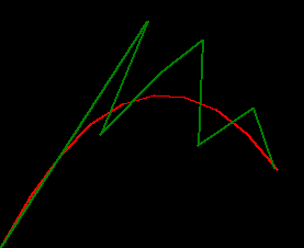
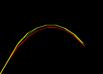
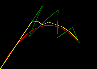
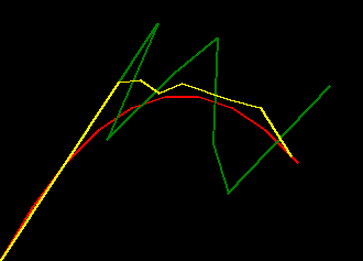
if we plot some examples of the default_params versus these trained params for
a range of missing_rate we can see the trained filter is much more robust to missing values
- red represents ground truth
- green represents the filter behaviour with the default params
- yellow represents the filter behaviour with the trained params
xy_trues = simulate_throw_a(3, 5)
seed = 1234414

def throw_img(xy_trues, seed, missing_rate):
  xy_preds_initial_params = rolled_out_predict_then_update(default_params(), seed, xy_trues, missing_rate)
  xy_preds_trained_params = rolled_out_predict_then_update(params, seed, xy_trues, missing_rate)
  return draw_throw_with_colours(
      [xy_trues, xy_preds_initial_params, xy_preds_trained_params],
      ['red',    'green',                 'yellow'])
 |
 |
 |
| missing_rate=0.0 | missing_rate=0.2 | missing_rate=0.4 |
how do the optimised params differ?
let's look at the differences between the original params and the ones that were learnt....
| param | original | learnt |
|---|---|---|
| A | [[1. 0. 1. 0.] [0. 1. 0. 1.] [0. 0. 1. 0.] [0. 0. 0. 1.]] |
[[ 0.958 0.014 0.897 0.038] [ 0.024 1.016 0.021 1.020] [ 0.004 -0.019 0.967 -0.003] [-0.026 -0.020 0.024 1.025]] |
| Q | [[0.25 0. 0.5 0. ] [0. 0.25 0. 0.5 ] [0.5 0. 1. 0. ] [0. 0.5 0. 1. ]] |
[[ 0.278 0.064 0.470 -0.035] [-0.001 0.279 0.013 0.513] [ 0.504 -0.027 1.031 0.042] [-0.002 0.465 0.003 1.005]] |
| R | [[0.01 0. ] [0. 0.01]] |
[[0.069 0.029] [0.011 0.137]] |
we can see that A and Q had minor changes but R was changed much more, particularly the value
related to y_std_meas
but what are we actually optimising?
seeing this result made me realise something. by providing the full A matrix to be optimised
we end up with non-zero and non-one values where as i really only wanted to tune for dt
it is interesting that the model has tuned the transistion matrix fully
but maybe in some cases it's better to constrain things and only allow it to change dt
to do this we just need to be more explict about what the actual parameter set is..
def default_params():
  return {
    'dt': 1.0,
    'std_acc': 1.0,
    'x_std_meas': 0.1,
    'y_std_meas': 0.1
  }
and then materialise A, Q and R from the params as required in predict and update
def predict(params, state):
  dt = params['dt']
  # State Transition Matrix
  A = jnp.array([[1, 0, dt, 0],
                 [0, 1, 0, dt],
                 [0, 0, 1, 0],
                 [0, 0, 0, 1]])
  # Process Noise Covariance
  Q = jnp.array([[(dt**4)/4, 0, (dt**3)/2, 0],
                 [0, (dt**4)/4, 0, (dt**3)/2],
                 [(dt**3)/2, 0, dt**2, 0],
                 [0, (dt**3)/2, 0, dt**2]]) * params['std_acc']**2

  state['x'] = A @ state['x']
  state['P'] = ((A @ state['P']) @ A.T) + Q
  xy_pred = state['x'][0]
  return state, xy_pred

def update(params, state, z):
  # Define Measurement Mapping Matrix
  H = jnp.array([[1, 0, 0, 0],
                 [0, 1, 0, 0]])
  # Measurement Noise Covariance
  R = jnp.array([[params['x_std_meas'] **2, 0],
                 [0, params['y_std_meas'] **2]])

  S = (H @ (state['P'] @ H.T)) + R
  K = (state['P'] @ H.T) @ jnp.linalg.inv(S)
  state['x'] = state['x'] + (K @ (z - (H @ state['x'])))
  I = jnp.eye(4)
  state['P'] = (I - (K @ H)) @ state['P']
  return state
doing this makes for a minor difference in the loss, and it's not really even visible in the trace visualisation.
to be honest though given the instability of the loss there are bigger things at play here in terms of ways to improve...
| step | full matrix params | scalar params |
|---|---|---|
| 0 | 2.561 | 5.138 |
| 100 | 12.69 | 24.98 |
| 200 | 4.009 | 2.928 |
| 300 | 4.407 | 6.072 |
| 400 | 4.803 | 2.422 |
| 500 | 3.536 | 2.577 |
| 600 | 3.029 | 4.388 |
| 700 | 2.361 | 3.006 |
| 800 | 3.024 | 1.631 |
| 900 | 1.736 | 3.306 |
some extensions
jax.vmap
running an update step per example is often troublesome. not only is it slow (since we're not making use of as much vectorisation as possible) it can also suffer a lot from gradient variance problems.
the general approach is to batch things and calculate gradients with respect to multiple examples before an update step. jax.vmap is perfect for this...
we can express the loss with respect to multiple examples by using jax to make a version of the rollout function that rolls out multiple trajectories at once...
note: in_axes denotes we want to vmap transform to vectorise over the
second and third arg of the loss function ( seed & xy_trues )
while broadcasting the first and last arg ( params & missing_rate )
def loss_fn(params, seeds, xy_truess, missing_rate):
  v_rolled_out_predict_then_update = jax.vmap(rolled_out_predict_then_update, in_axes=[None, 0, 0, None])
  predictions = v_rolled_out_predict_then_update(params, seeds, xy_truess, missing_rate)
  squared_difference = (predictions - xy_truess) ** 2
  return jnp.mean(squared_difference)
this loss is called as before but instead with a batch of seeds and xy_trues
batch_size = 8
xy_truess = []
seeds = []
for _ in range(batch_size):
  dx = 2 + np.random.uniform() * 5  # (2, 7)
  dy = 4 + np.random.uniform() * 4  # (4, 8)
  xy_truess.append(simulate_throw_a(dx, dy))
  seeds.append(next_seed)
  next_seed += 1
xy_truess = np.stack(xy_truess)
seeds = np.array(seeds)
...
params = update_step(params, seeds, xy_truess)
interestingly i found this didn't actually help! usually for a neural network this is a big win, for speed as well as gradient variance, but in this case it was behaving worse for me :/
why you no optax?
rolling your own optimisation step is generally (*) a bad idea, better to use an update step using an optax optimiser.
params = default_params()
opt = optax.adam(1e-6)
opt_state = opt.init(params)
...
@jax.jit
def update_step(params, opt_state, seeds, xy_truess):
  gradients = jax.grad(loss_fn)(params, seeds, xy_truess, missing_rate=0.1)
  updates, opt_state = opt.update(gradients, opt_state)
  params = optax.apply_updates(params, updates)
  return params, opt_state
...
for i in range(1000):
  ...
  params, opt_state = update_step(params, opt_state, seeds, xy_truess)
  ...
having said that trying a couple of different optimisers gave no better result than the simple hand rolled update step from above!!! i guess the dynamics are weird enough that they aren't fitting the expected default space of adam, rmsprop, etc (?) am betting on the noisy behaviour of the rollout to be at fault...
cross product of possible data
sometimes the best way to avoid noisy samples is go nuts on a fixed large dataset size
e.g. if we just materialise a large range of cross product values for dx, dy ...
N = 40
SEEDS_PER_DX_DY = 50
xy_truess = []
seeds = []
for dx_l in np.linspace(0, 1, N):
  for dy_l in np.linspace(0, 1, N):
    xy_trues = simulate_throw_a(dx=2+(dx_l*5), dy=4+(dy_l*4))
    for _ in range(SEEDS_PER_DX_DY):
      xy_truess.append(xy_trues)
xy_truess = np.stack(xy_truess)
seeds = np.array(range(len(xy_truess)))
print("xy_truess", xy_truess.shape, "seeds", seeds.shape)
xy_truess (80000, 10, 2) seeds (80000,)
we can then jit this fixed data into the update step
@jax.jit
def update_step(params, opt_state):
  gradients = jax.grad(loss_fn)(params, seeds, xy_truess, missing_rate=0.1)
  updates, opt_state = opt.update(gradients, opt_state)
  params = optax.apply_updates(params, updates)
  return params, opt_state

for i in range(1000):
  params, opt_state = update_step(params, opt_state)
  if i % 100 == 0:
    print("loss", i, loss_fn(params, seeds, xy_truess, missing_rate=0.1))
and we get a fast update and the most stable loss, though it flattens out pretty quick
loss 0 9.521738
loss 100 5.65931
loss 200 5.651896
loss 300 5.6428213
loss 400 5.636997
...
| variable | initial | trained |
|---|---|---|
| dt | 1.0 | 1.3539 |
| std_acc | 1.0 | 0.1803 |
| x_std_meas | 0.1 | 0.1394 |
| y_std_meas | 0.1 | 0.1 |
curiously in this formulation we've ended up with no gradients with respect to y_std_meas (?)
so i've either got a bug or it's the subtle way it's being used.. TODO!
anyways, that's my time up. check out the prototype colab i made for this post