tl;dr

random embedding networks can be used to generate weakly labelled data for metric learning and they see a large benefit from being run in ensembles.

can we represent these ensembles as a single forward pass in jax? why yes! yes we can!

overview

a fundamental question when training embedding models is deciding how to specify the examples we want to be close vs examples we want to be far apart.

consider a collection of renders of random synthetic objects that look something like...

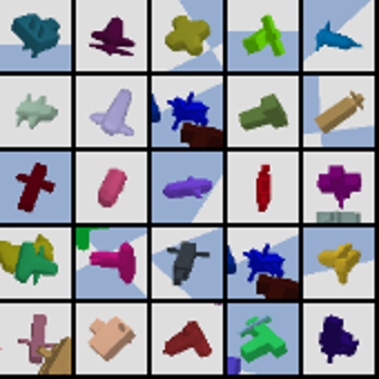
( check out my minimal example of running pybullet under google cloud dataflow if you'd like to generate a large amount of your own )

can we train an model that learns embeddings for these objects without explicit labels? i.e. is there a way of weakly labelling these? yes! by using random embedding networks.

it turns out if we just initialise (don't train!) an embedding network that images of the same object will sometimes be embedded closest to each other. we can use this as a form of weak labelling; it just has to occur more often than random.

consider a collage of 3 "test examples" with each example consisting of 11 images.

• first column: an anchor image which is a random render of a random object.
• second column: a positive image which is another render of the same object.
• 9 remaining column: negative images which are renders of other objects.

though this collage shows 3 examples the full test set we'll be using will contain N=100 examples

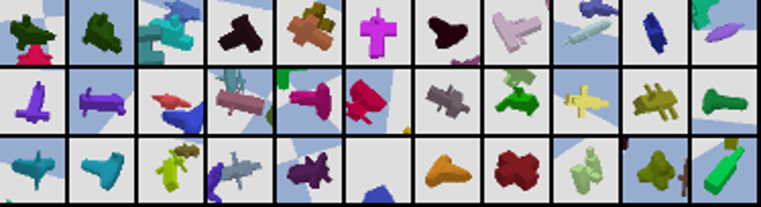
we can quantify the quality of a random embedding network by embedding all 11 of these images and seeing how often the anchor is closer to the positive than any of the negatives. given there are 9 negatives for each positive we know that random choice accuracy would be 0.1. the question is then, can we do better with random embeddings?

code

to repro all this have a look at this far less commented colab

first let's get some pre cooked test data ...

>>> !wget "https://github.com/matpalm/shared_data/blob/master/test_set_array.npy.gz?raw=true" -O test_set_array.npy.gz --quiet
>>> !gunzip -f test_set_array.npy.gz
>>>
>>> test_set_array = np.load("test_set_array.npy")
>>> N = test_set_array.shape[0]  # number of examples in test set

this array is shaped (N, 11, HW, HW, 3); and again, as before

• N = 100 represents the 100 test set examples.
• 11 represents the anchor, positive & 9 negatives.
• (HW, HW, 3) represents the image tensor

a random embedding keras model

let's start with a basic keras model. this model is taken from another one of my projects and forms the basis of a fully convolutional network. in this form it is structured to have a convolutional stack that takes an input of (32, 32, 3) and outputs a (1, 1, 256) spatial feature map. this feature map is passed through a Dense layer with ReLU activation (implemented as a 1x1 convolution) followed by a linear projection to a E dimensional embedding. we normalise the embeddings to unit length for ease of the upcoming similarity calculations.

>>> E = 32   # output embedding dimension used for all models
>>>
>>> class NormaliseLayer(Layer):
>>>     def call(self, x):
>>>         return tf.nn.l2_normalize(x, axis=-1)
>>>
>>> def conv(x, filters):
>>>     return Conv2D(filters=filters, kernel_size=3, strides=2,
>>>                   padding='VALID', kernel_initializer='orthogonal',
>>>                   activation='relu')(x)
>>>
>>> def construct_model():
>>>     inputs = Input(shape=(HW, HW, 3))
>>>     model = conv(inputs, 32)
>>>     model = conv(model, 64)
>>>     model = conv(model, 128)
>>>     model = conv(model, 256)
>>>     model = Dense(units=32, kernel_initializer='orthogonal',
>>>                   activation='relu')(model)
>>>     embeddings = Dense(units=E, kernel_initializer='orthogonal',
>>>                       activation=None, name='embedding')(model)
>>>     embeddings = NormaliseLayer()(embeddings)
>>>     return Model(inputs, embeddings)
>>>
>>> model = construct_model()
>>> model.summary()

    _________________________________________________________________
    Layer (type)                 Output Shape              Param #
    =================================================================
    input_1 (InputLayer)         [(None, 32, 32, 3)]       0
    conv2d (Conv2D)              (None, 15, 15, 32)        896
    conv2d_1 (Conv2D)            (None, 7, 7, 64)          18496
    conv2d_2 (Conv2D)            (None, 3, 3, 128)         73856
    conv2d_3 (Conv2D)            (None, 1, 1, 256)         295168
    dense (Dense)                (None, 1, 1, 32)          8224
    embedding (Dense)            (None, 1, 1, 32)          1056
    normalise_layer (NormaliseLa (None, 1, 1, 32)          0
    =================================================================
    Total params: 397,696
    Trainable params: 397,696
    Non-trainable params: 0

we'll need some utility functions to

1. run images through this model...
2. calculate the cosine sims between the different types of the embeddings and
3. calculate an overall accuracy for the 100 test examples.

>>> def embeddings_for(model, imgs):
>>>     embeddings = model.predict(imgs.reshape(N*11, HW, HW, 3))
>>>     return embeddings.reshape(N, 11, E)
>>>
>>> def anc_pos_neg_sims(embeddings):
>>>     # slice anchors, positives and negatives out of embeddings
>>>     # and calculate pair wise sims using dot product similarity.
>>>     # returns (N, 10) representing N examples of anchor compared to
>>>     # positives / negatives.
>>>     anchor_embeddings = embeddings[:, 0]              # (N, E)
>>>     positive_negative_embeddings = embeddings[:, 1:]  # (N, 10, E)
>>>     return np.einsum('ne,npe->np', anchor_embeddings,
>>>                      positive_negative_embeddings)    # (N, 10)
>>>
>>> def accuracy(sims):
>>>     # given a set of (N, 10) sims calculate accuracy. note that the data has
>>>     # been prepared such that correct element is the 0th element so accuracy
>>>     # is simply the times the most similar is the 0th.
>>>     most_similar = np.argmax(sims, axis=1)
>>>     times_correct = sum(most_similar == 0)
>>>     return times_correct / N
>>>
>>> accuracy(anc_pos_neg_sims(embeddings_for(model, test_set_array)))

0.26

( note: if you're new to einsum check out my illustrative einsum example explainer video where i walk through what the einsum operations in this post are doing )

great! this model does (slightly) better than random (which would have been 0.1). hooray!

since this model isn't even trained, we should expect a degree of variance across a number of differently initialised models. let's build M=10 models and see how things vary.

>>> M = 10  # number of models to run in ensemble
>>>
>>> models = [construct_model() for _ in range(M)]
>>> per_model_sims = np.stack([anc_pos_neg_sims(embeddings_for(m, test_set_array)) for m in models])  # (M, N, 10)
>>> accuracies = [accuracy(sims) for sims in per_model_sims]
>>>
>>> print("accuracies", accuracies)
>>> print("mean", np.mean(accuracies), "std", np.std(accuracies))

accuracies [0.2, 0.29, 0.26, 0.29, 0.29, 0.26, 0.29, 0.26, 0.27, 0.32]
mean 0.273 std 0.03034798181098703

an ensemble?

given this amount of variance we can ask, how would an ensemble do? a great thing about the way this model is structured is that we can do a weighted ensemble in a really simple way.

note that the prediction is based on the argmax of these similarities, this means to combine them in an ensemble all we need to do is sum them before the argmax!

since the embeddings are unit length the cosine similarity is being constrained to (-1, 1). so when we sum them what we're doing is taking a form of weighted vote. nice!

>>> accuracy(np.sum(per_model_sims, axis=0))

0.4

great! the weighted ensemble does noticably better than any of the individual random models (which in turn did better than random choice)

but it feels a bit clumsy to have to run these M models sequentially. could we model this directly in a pass of a single network?

what is input batching doing?

let's think about what batching inputs does;

the simplest form of a model takes an input, applies some layers parameterised in some way (by theta here) to calculate some hidden layer values and finally produces an output.

\( I \rightarrow f^1(\theta^1) \rightarrow H \rightarrow f^2(\theta^2) \rightarrow O \)

what we almost always do though is run a batch of B examples through at a time. batching inputs allows us to make the best use of hardware acceleration, as well as getting use some theoretical benfits regarding optimisation. since we're using the same model we have a single set of thetas and we produce a batch of B outputs.

\( I_B \rightarrow f^1(\theta^1) \rightarrow H_B \rightarrow f^2(\theta^2) \rightarrow O_B \)

but what we want to do now is to not just have a batch of B inputs, but also a batch of M models as well.

\( I_B \rightarrow f^1(\theta^1_M) \rightarrow H_{B,M} \rightarrow f^2(\theta^2_M) \rightarrow O_{B,M} \)

though the algebra is no different this idea of having multiple sets of theta for a layer isn't something that naturally fits in the standard frameworks. :( maybe this is something you could get going with keras but the couple of attempts i tried met heavy framework resistance :/ perhaps this functionality of arbitrary mapping seems a good fit for jax's vmap; but how would it work?

a random embedding jax model

first let's rebuild this network in a minimal way with jax but without any layer framework. not using a layer framework means we'll need to maintain our own set of model parameters. note that we for this model we're not going to bother with bias terms, they would be zero by initialisation anyways (we're remember not training at all, just building and running these networks)

note we also more explicitly refer to the dense layer here as using a 1x1 kernel convolution. this is actually equivalent to what's happening the above keras model where a Dense layer on a (H, W, C) input automagically does things as a 1x1 convolution.

>>> key = random.PRNGKey(0)
>>> _key, *subkeys = random.split(key, 7)
>>>
>>> params = {
>>>   'conv1_kernel': orthogonal()(subkeys[0], (3, 3, 3, 32)),
>>>   'conv2_kernel': orthogonal()(subkeys[1], (3, 3, 32, 64)),
>>>   'conv3_kernel': orthogonal()(subkeys[2], (3, 3, 64, 128)),
>>>   'conv4_kernel': orthogonal()(subkeys[3], (3, 3, 128, 256)),
>>>   'dense_kernel': orthogonal()(subkeys[4], (1, 1, 256, 32)),
>>>   'embedding_kernel': orthogonal()(subkeys[5], (1, 1, 32, 32))
>>> }
>>>
>>> conv_dimension_numbers = lax.conv_dimension_numbers((1, HW, HW, 3),  # input shape prototype
>>>                                                     (3, 3, 1, 1),    # 2d kernel shape prototype
>>>                                                     ('NHWC',         # input
>>>                                                      'HWIO',         # kernel
>>>                                                      'NHWC'))        # output
>>>
>>> def conv_block(stride, with_relu, input, kernel):
>>>     no_dilation = (1, 1)
>>>     block = lax.conv_general_dilated(input, kernel, (stride, stride), 'VALID',
>>>                                      no_dilation, no_dilation,
>>>                                      conv_dimension_numbers)
>>>     if with_relu:
>>>         block = relu(block)
>>>     return block
>>>
>>> @jit
>>> def model(params, input):                                                         # (N, 32, 32, 3)
>>>     conv1_output = conv_block(2, True, input, params['conv1_kernel'])             # (N, 15, 15, 32)
>>>     conv2_output = conv_block(2, True, conv1_output, params['conv2_kernel'])      # (N, 7, 7, 64)
>>>     conv3_output = conv_block(2, True, conv2_output, params['conv3_kernel'])      # (N, 3, 3, 128)
>>>     conv4_output = conv_block(2, True, conv3_output, params['conv4_kernel'])      # (N, 1, 1, 256)
>>>     dense1_output = conv_block(1, True, conv4_output, params['dense_kernel'])     # (N, 1, 1, E)
>>>     embeddings = conv_block(1, False, dense1_output, params['embedding_kernel'])  # (N, 1, 1, E)
>>>     embeddings /= jnp.linalg.norm(embeddings, axis=-1, keepdims=True)             # (N, 1, 1, E)
>>>     return embeddings

in terms of utility functions we can reuse the above anc_pos_neg_sims and accuracy from before but we'll need to change the embeddings_for slightly based on how jax and keras models are called differently.

>>> def embeddings_for(params, imgs):
>>>     embeddings = model(params, imgs.reshape(N*11, HW, HW, 3))
>>>     return embeddings.reshape(N, 11, E)
>>>
>>> accuracy(anc_pos_neg_sims(embeddings_for(params, test_set_array)))

0.27

a single network ensemble?

ok, a single random model does about the same. that helps give us confidence there's no weird behaviour difference the keras and the jax model. next, how do we handle the ensemble idea in a single network?

firstly we need to remake all the kernels but with a leading M dimension that represents the M models we want to run in parallel.

>>> key = random.PRNGKey(0)
>>> _key, *subkeys = random.split(key, 7)
>>>
>>> params = {
>>>   conv1_kernels = orthogonal()(subkeys[0], (M, 3, 3, 3, 32)),
>>>   conv2_kernels = orthogonal()(subkeys[1], (M, 3, 3, 32, 64)),
>>>   conv3_kernels = orthogonal()(subkeys[2], (M, 3, 3, 64, 128)),
>>>   conv4_kernels = orthogonal()(subkeys[3], (M, 3, 3, 128, 256)),
>>>   dense_kernels = orthogonal()(subkeys[4], (M, 1, 1, 256, 32)),
>>>   embedding_kernels = orthogonal()(subkeys[5], (M, 1, 1, 32, 32))
>>> }

and then all we have to do is run the same model as before, but using vmap for the calls. we use in_axes to denote we want to vectorise over the 0th index of the first arg (the params) but want don't want to vectorise over the second arg (the imgs)

>>> vmap_model = jit(vmap(model, in_axes=(0, None)))

for the final example of running this model we forgo the previous utility functions and run each step explicitly.

first we run the images through the model. this produces a (M, N, 11, E) output instead of a (N, 11, E) output as before.

>>> embeddings = vmap_model(params, test_set_array.reshape(N*11, HW, HW, 3))
>>> embeddings = embeddings.reshape((M, N, 11, E))
>>> embeddings.shape

(10, 100, 11, 32)

next we slice out the anchors from the positives and negatives

>>> anchor_embeddings = embeddings[:, :, 0]                         # (M, N, E)
>>> positive_negative_embeddings = embeddings[:, :, 1:]             # (M, N, 10, E)

we can calculate the per model accuracy by doing the reducing and explicitly keeping m in the output.

>>> per_model_sims = jnp.einsum('mne,mnpe->mnp',
>>>                             anchor_embeddings,
>>>                             positive_negative_embeddings)        # (M, N, 10)
>>>
>>> most_similar = jnp.argmax(per_model_sims, axis=2)    # (10, N)
>>> times_correct = jnp.sum(most_similar == 0, axis=1)   # (10,)
>>> accuracies = times_correct / N                       # (10,)
>>> accuracies

array([0.25, 0.29, 0.24, 0.23, 0.21, 0.25, 0.3 , 0.25, 0.27, 0.31])

cool. so each model has some degree of variance, as the keras models did.

finally we can represent the ensemble by simply doing a further reduction over m in the einsum calculation.

>>> ensemble_sims = jnp.einsum('mne,mnpe->np',
>>>                            anchor_embeddings,
>>>                            positive_negative_embeddings)       # (N, 10)
>>>
>>> most_similar = jnp.argmax(ensemble_sims, axis=1)  # (N,)
>>> times_correct = jnp.sum(most_similar == 0)        # (1,)
>>> accuracy = times_correct / N                      # (1,)
>>> accuracy

DeviceArray(0.4, dtype=float32)

all this required only one forward pass through a single model, and with the weighted voting idea of the ensemble, we only required an extra m reduction in einsum sims call. so elegant!