<<  take 2: term frequency    index    part 4: but does it scale?  >>

take 3: markov chains

sip_markov

using term frequency was a good start but it relies too much on all the terms being infrequent which is not really that fair. for example given the 'stop your jibber and jabber man!' we might like to conclude that 'jibber and jabber' is a reasonable sip even though it includes a common word like 'and'.

what we need is a way to take into account the sequence of words, and markov chains are a great way to do this. i've talked about , before in other experiments (eg this one) so go have a read if you're new to them.

let's ignore term frequencies completely and trying using a markov chain to find the sips

consider the sequence of characters
abaabdabaabdabaabdacdbacd
( the astute reader might notice this is the string 'abaabd'*3 + 'acdbacd' contrived to have 'c' as a rare character and 'a' as a common one )

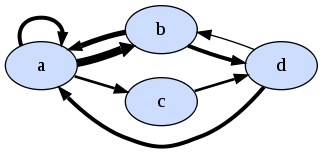
considering character to character transistion we can build the markov chain

a -> a = 3/11 (0.27) (ie 'a' appears 11 times and is followed by 'a' 3 of those times)
a -> b = 6/11 (0.55)
a -> c = 2/11 (0.18)
b -> a = 4/7 (0.57)
b -> d = 3/7 (0.43)
c -> d = 2/2 (1.00)
d -> a = 3/4 (0.75)
d -> b = 1/4 (0.25)

we can define sip_markov(abc) = p(a->b) * p(b->c)
eg from the above markov chain

p(dab) = p(d->a) * p(a->b) = 0.750 * 0.545 = 0.409
p(bac) = p(b->a) * p(a->c) = 0.571 * 0.182 = 0.104 

calculating sip_markov for all trigram sequences we get...

dab = da * ab = 0.750 * 0.545 = 0.409
bda = bd * da = 0.429 * 0.750 = 0.321 
aba = ab * ba = 0.545 * 0.571 = 0.312 
cdb = cd * db = 1.000 * 0.250 = 0.250 
abd = ab * bd = 0.545 * 0.429 = 0.234 
acd = ac * cd = 0.182 * 1.000 = 0.182 
baa = ba * aa = 0.571 * 0.273 = 0.156 
aab = aa * ab = 0.273 * 0.545 = 0.149 
dba = db * ba = 0.250 * 0.571 = 0.143 
dac = da * ac = 0.750 * 0.182 = 0.136 
bac = ba * ac = 0.571 * 0.182 = 0.104 

it's interesting to note that acd and cdb are quite high when they shouldn't really be since both c and d are rarish characters. why is this?

since c is always followed by d and markov chain's are only concerned with the transistions it results in a mulitplier of 1, even though c is very rare.

so it looks like we need a combination of both the transistion probabilities from the markov chain and the term frequency probabilities.

combining sip_mle with sip_markov

how might we define a combined metric sip_combined(abc) in terms of sip_mle('abc') and sip_markov('abc')?

recall sip_mle('abc') = p(a) * p(b) * p(c) and sip_markov('abc') = p(a -> b) * p(b -> c)

i started by using the geometric mean which seemed a natural choice.

sip_combined('abc') = √ ( sip_mle('abc') * sip_markov('abc') )

here is the derivation of an variation on the geometric mean that weighted the components differently. i use == to denote an operation that produces a value that will retain order since we only really care about finding the least probable without caring about the exact values

sip_combined('abc') 
 = √ ( sip_mle('abc') * sip_markov('abc') )
== sip_mle('abc') * sip_markov('abc') 
 = p(a) * p(b) * p(c) * p(a -> b) * p(b -> c)
 = e ^ ( ln(p(a)) + ln(p(b)) + ln(p(c)) + ln(p(a -> b)) + ln(p(b -> c)) )
== ln(p(a)) + ln(p(b)) + ln(p(c)) + ln(p(a -> b)) + ln(p(b -> c))  
 = x + y + z + u + v   # save some writing
== mean(x, y, z, u, v)

sip_combined('abc') 
 = mean( mean(x, y, z), mean(u, v) )
== mean(x, y, z) + mean(u, v) 

an example, please....

term probabilities are

a 11/25 == ln(11/25) = -0.82
b 7/25  == ln(7/25)  = -1.27
d 5/25  == ln(5/25)  = -1.60
c 2/25  == ln(2/25)  = -2.52

and recall markov chain probabilities are

a -> a = 3/11 == ln(3/11) = -1.29
a -> b = 6/11 == ln(6/11) = -0.60
a -> c = 2/11 == ln(2/11) = -1.70
b -> a = 4/7  == ln(4/7)  = -0.55
b -> d = 3/7  == ln(3/7)  = -0.84
c -> d = 2/2  == ln(2/2)  =  0.00
d -> a = 3/4  == ln(3/4)  = -0.28
d -> b = 1/4  == ln(1/4)  = -1.38

bac = (-1.273 -0.821 -2.526)/3 + (-0.560 -1.705)/2 = -4.620/3 -2.264/2 = -2.672
dac = (-1.609 -0.821 -2.526)/3 + (-0.288 -1.705)/2 = -4.956/3 -1.992/2 = -2.648
acd = (-0.821 -2.526 -1.609)/3 + (-1.705 -0.000)/2 = -4.956/3 -1.705/2 = -2.504
dba = (-1.609 -1.273 -0.821)/3 + (-1.386 -0.560)/2 = -3.703/3 -1.946/2 = -2.207
abd = (-0.821 -1.273 -1.609)/3 + (-0.606 -0.847)/2 = -3.703/3 -1.453/2 = -1.961
aab = (-0.821 -0.821 -1.273)/3 + (-1.299 -0.606)/2 = -2.915/3 -1.905/2 = -1.924
baa = (-1.273 -0.821 -0.821)/3 + (-0.560 -1.299)/2 = -2.915/3 -1.859/2 = -1.901
bda = (-1.273 -1.609 -0.821)/3 + (-0.847 -0.288)/2 = -3.703/3 -1.135/2 = -1.802
dab = (-1.609 -0.821 -1.273)/3 + (-0.288 -0.606)/2 = -3.703/3 -0.894/2 = -1.681

building the markov chain

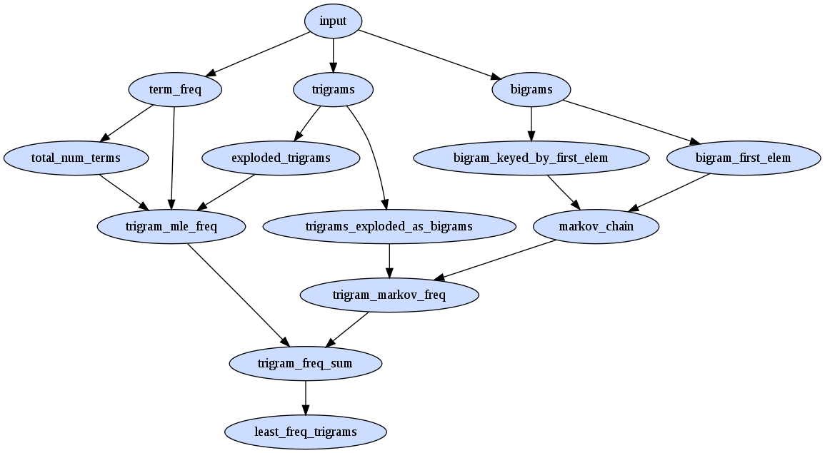
finally how did will we generate the markov chain using map reduce semantics? it's actually very similiar to the task required for building the term frequencies

consider abacabc
we want a markov chain

a > b 2/3
a > c 1/3
b > a 1/2
b > c 1/2
c > a 1/1

first off we need the frequencies of bigrams, and a version of them keyed by the first term. these values make up the nominators of the transistion probabilites in the chain

bash> rake bigrams
bash> rake cat dir=bigrams
ab  2
ac  1
ba  1
bc  1
ca  1
bash> rake bigram_keyed_by_first_elem
bash> rake cat dir=bigram_keyed_by_first_elem
a.1f  ab 2
a.1f  ac 1
b.1f  ba 1
b.1f  bc 1
c.1f  ca 1

then we need the frequencies of the 'from' state. these values make up the denominators of the transistion probabilites in the chain

bash> rake bigram_first_elem
bash> rake cat dir=bigram_first_elem
a.0p 3
b.0p 2
c.0p 1

we can them join these last two

bash> rake markov_chain
bash> rake cat dir=markov_chain
ab.0p  0.66
ac.0p  0.33
ba.0p  0.5
bc.0p  0.5
ca.0p  1

once we have our markov chain model we can join it to the trigrams in a similiar fashion to how we joined the term frequencies with the trigrams on the last page

here's the new set of map reduce passes required...

the bigger example

how does the inclusion of markov_sip change the sips on our 8 document corpus?

doc	sip1	sip2	sip3
fbncc10	and numbers edited	university of quebec	structure in 2000
8sknn10	think a scrimption	by she noiselessly	he been disgusted
gm77v10	he the venom	the not colloquial	the not unamiable
7hmvg10	for on dormant	and english morello	to deep carmine
dwqoh10	thinks and nobobody	when one watches	the indifferent routinists
7stir10	or la nouvelle	to poor ellen	poor of marlowe
esper10	in out ow	a old maljunec	in day aye
8prmt10	de by belmekhira	in die ferse	sie in feierlichem

sort of interesting... there are some further improvements that could be made;

1. take an tfidf approach in that you should favour combos that appear a lot in a particular document
2. allow bigrams not just trigrams, which with the previous approach will pluck out bits of terminology

but does it scale?

<<  take 2: term frequency    index    part 4: but does it scale?  >>

sept 2009