


brain of mat kelcey...
pseudocounts and the good-turing estimation (part1)
April 03, 2011 at 03:04 PM | categories: Uncategorizedbeer
say we are running the bar at a soldout bad religion concert. the bar serves beer, scotch and water and we decide to record orders over the night so that we can know how much to order for tomorrow's gig...
| drink | #sales |
| beer | 1000 |
| scotch | 300 |
| water | 200 |
using these numbers we can predict a number of things..
what is the chance the next person will order a beer? it's a pretty simple probability; 1000 beers / 1500 total drinks = 0.66 or 66%
what is the chance the next person will order a water? also straightforward; 200 waters / 1500 total drinks = 0.14 or 14%
t-shirts
now say we run the t-shirt stand at the same concert....
instead of only selling 3 items (like at the bar) we sell 20 different types of t-shirts. once again we record orders over the night...
| t-shirt | #sales | t-shirt | #sales |
| br tour | 15 | pennywise | 3 |
| br logo1 | 15 | strung out | 3 |
| br album art 1 | 10 | propagandhi | 3 |
| br album art 3 | 10 | bouncing souls | 1 |
| nofx logo1 | 5 | the vandals | 1 |
| nofx logo2 | 5 | dead kennedys | 1 |
| lagwagon | 4 | misfits | 1 |
| frenzal rhomb | 4 | the offspring | 0 |
| rancid | 4 | the ramones | 0 |
| descendants | 3 | mxpx | 0 |
we can ask similar questions again regarding the chance of people buying a particular t-shirt
what's the chance the next person to buy a t-shirt wants the official tour t-shirt? 15 tour t-shirts sold / 88 sold in total = 0.170 or 17.0%
what's the chance the next person to buy a t-shirt wants the a descendants t-shirt? 3 descendants t-shirts sold / 88 sold in total = 0.034 or 3.4%
what's the chance the next person to buy a t-shirt wants the an offspring t-shirt? 0 offspring t-shirts sold / 88 sold in total = 0 or 0%
if you're like me then the last one "feels" wrong. even though we've not seen a purchase of at least 1 t-shirt it seems a bit rough to say there is no chance of someone buying one. this illustrates one of the problems of dealing prior probabilities
any system using a products of probabilities, such as the modeling of "independent" events in naive bayes, suffers badly from these zero probabilities. i've discussed the problems a few times before in previous experiments such as (this one on naive bayes and this one on semi supervised bayes) and the approach i've always used is the simple rule of succession where we avoid the zero problem by adding one to the frequency of each event.
for reference here are the probabilities per t-shirt without adjustment...
R> sales = rep(c(15,10,5,4,3,1,0), c(2,2,2,3,4,4,3))
 [1] 15 15 10 10  5  5  4  4  4  3  3  3  3  1  1  1  1  0  0  0
R> simple_probs = sales / sum(sales)
 [1] 0.17045455 0.17045455 0.11363636 0.11363636 0.05681818 0.05681818
 [7] 0.04545455 0.04545455 0.04545455 0.03409091 0.03409091 0.03409091
[13] 0.03409091 0.01136364 0.01136364 0.01136364 0.01136364 0.00000000
[19] 0.00000000 0.00000000
... and here are the values for the succession rule case
R> sales = rep(c(15,10,5,4,3,1,0), c(2,2,2,3,4,4,3))
 [1] 15 15 10 10  5  5  4  4  4  3  3  3  3  1  1  1  1  0  0  0
R> sales_plus_one = sales + 1
 [1] 16 16 11 11  6  6  5  5  5  4  4  4  4  2  2  2  2  1  1  1
R> smooth_probs = sales_plus_one / sum(sales_plus_one)
 [1] 0.14814815 0.14814815 0.10185185 0.10185185 0.05555556 0.05555556
 [7] 0.04629630 0.04629630 0.04629630 0.03703704 0.03703704 0.03703704
[13] 0.03703704 0.01851852 0.01851852 0.01851852 0.01851852 0.00925926
[19] 0.00925926 0.00925926
no more zeros! yay! but, unfortunately, at the cost of the accuracy of the other values.
it's always worked for me in the past (well at least better than having the zeros) but it's always felt wrong too. but finally the other day i found another approach, that seems a lot more statistically sound.
it's called good-turing estimation and it was developed as part of turing's work at bletchley park (so it must be awesome). a decent implementation is explained in this paper by geoffrey sampson (it's somewhat more complex than adding 1)
it works on using the frequency of frequencies and redistributes the probabilities to include a special allocation that we should allocate over items that have never seen before.
the following table shows the frequencies, the original probability, the probability adjusted using the rule of succession and the probabilities as redistributed using good turing estimation.
| freq | freq of freq | originalprob | successionprob | good turingprob | description |
| 15 | 2 | 0.170 | 0.148 | 0.160 | 2 t-shirts sold 15 times |
| 10 | 2 | 0.113 | 0.101 | 0.107 | 2 t-shirts sold 10 times |
| 5 | 2 | 0.056 | 0.055 | 0.054 | 2 t-shirts sold 5 times |
| 4 | 3 | 0.045 | 0.046 | 0.043 | 3 t-shirts sold 4 times |
| 3 | 4 | 0.034 | 0.037 | 0.033 | 4 t-shirts sold 3 times |
| 1 | 4 | 0.011 | 0.018 | 0.011 | 4 t-shirts sold once |
| 0 | 3 | 0.000 | 0.009 | 0.015 | 3 t-shirts didn't sell |
and here's a graph of the same thing.
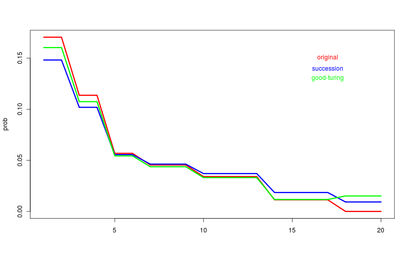
some observations...
- the rule as succession is just smoothing really and drags the higher probabilities down in response to pulling the lower probabilities up
- the good turing estimation is closer to the real value of the high frequency cases
- the good turing estimate for the zero case is quite a bit higher than the rule of succession estimate
- and most interesting of all, the good turing estimate for the freq 0 is higher than the estimate for freq 1.
the last point in particular i think is really interesting. the good turing algorithm actually gives a total estimate for the zero probability cases (in this examples it gave 0.045) and it's up to the user to distribute it among the actual examples (in this example there were 3 cases so i just divided 0.045 by 3).
if there had be 4 types of t-shirts that hadn't sold the estimate for each of them would have be 0.011 like the 4 t-shirts that sold once.
if there had only be 1 type of t-shirt that hadn't had any sales we'd have to allocate the entire 0.045 to it. in effect the algorithms says it expects that t-shirt to be more likely to sell that the 4 types of t-shirts that had 3 sales each (the 0.033 probability case).
an interesting result, not sure what intution to take away from it....
now this is all good, but i actually don't run the bar at a bad religion concert (or the t-shirt stand) and i'm actually interested in this in how it applies to text processing, especially in the area of classification.
so my question is "is the extra computation required for the good-turing calculation worth it?"
results coming in part2. work in progress code on github