brain of mat kelcey...

pymc / mcmc / mind blown

PyMC is a python library for working with bayesian statistical models, primarily using MCMC methods. as a software engineer who has only just scratched the surface of statistics this whole MCMC business is blowing my mind so i've got to share some examples.

fitting a normal

let's start with the simplest thing possible, fitting a simple distribution.

say we have a thousand values, 87.27, 67.98, 119.56, ... and we want to build a model of them.

a common first step might be to generate a histogram.

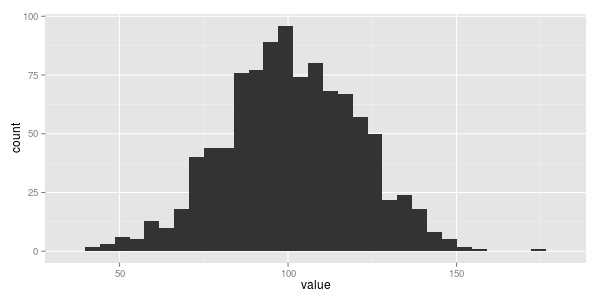
if i had to a make a guess i'd say this data looks normally distributed. somewhat unsurprising, not just because normal distributions are freakin everywhere, (this great khan academy video on the central limit theorem explains why) but because it was me who synthetically generated this data in the first place ;)

now a normal distribution is parameterised by two values; it's mean (technically speaking, the "middle" of the curve) and it's standard deviation (even more technically speaking, how "fat" it is) so let's use PyMC to figure out what these values are for this data.

!!warning!! !!!total overkill alert!!! there must be a bazillion simpler ways to fit a normal to this data but this post is about dead-simple-PyMC not dead-simple-something-else.

first a definition of our model.

# simple_normal_model.py
from pymc import *
data = map(float, open('data', 'r').readlines())
mean = Uniform('mean', lower=min(data), upper=max(data))
precision = Uniform('precision', lower=0.0001, upper=1.0)
process = Normal('process', mu=mean, tau=precision, value=data, observed=True)

working backwards through this code ...

• line 6 says i am trying to model some process that i believe is Normally distributed defined by variables mean and precision. (precision is just the inverse of the variance, which in turn is just the standard deviation squared). i've already observed this data and the values are in the variable data
• line 5 says i don't know the precision for my process but my prior belief is it's value is somewhere between 0.0001 and 1.0. since i don't favor any values in this range my belief is uniform across the values. note: assuming a uniform distribution for the precision is overly simplifying things quite a bit, but we can get away with it in this simple example and we'll come back to it.
• line 4 says i don't know the mean for my data but i think it's somewhere between the min and the max of the observed data. again this belief is uniform across the range.
• line 3 says the data for my unknown process comes from a local file (just-plain-python)

the second part of the code runs the MCMC sampling.

from pymc import *
import simple_normal_model
model = MCMC(simple_normal_model)
model.sample(iter=500)
print(model.stats())

working forwards through this code ...

• line 4 says build a MCMC for the model from the simple_normal_model file
• line 5 says run a sample for 500 iterations
• line 6 says print some stats.

and that's it!

the output from our stats includes among other things estimates for the mean and precision we were trying to find

{
'mean': {'95% HPD interval': array([  94.53688316,  102.53626478]) ... },
'precision': {'95% HPD interval': array([ 0.00072487,  0.03671603]) ... },
...
}

now i've brushed over a couple of things here (eg the use of uniform prior over the precision, see here for more details) but i can get away with it all because this problem is a trivial one and i'm not doing gibbs sampling in this case. the main point i'm trying to make is that it's dead simple to start writing these models.

one thing i do want to point out is that this estimation doesn't result in just one single value for mean and precision, it results in a distribution of the possible values. this is great since it gives us an idea of how confident we can be in the values as well as allowing this whole process to be iterative, ie the output values from this model can be feed easily into another.

deterministic variables

all the code above parameterised the normal distribution with a mean and a precision. i've always thought of normals though in terms of means and standard deviations (precision is a more bayesian way to think of things... apparently...) so the first extension to my above example i want to make is to redefine the problem in terms of a prior on the standard deviation instead of the precision. mainly i want to do this to introduce the deterministic concept but it's also a subtle change in how the sampling search will be directed because it introduces a non linear transform.

data = map(float, open('data', 'r').readlines())

mean = Uniform('mean', lower=min(data), upper=max(data))
std_dev = Uniform('std_dev', lower=0, upper=50)

@deterministic(plot=False)
def precision(std_dev=std_dev):
    return 1.0 / (std_dev * std_dev)

process = Normal('process', mu=mean, tau=precision, value=data, observed=True)

our code is almost the same but instead of a prior on the precision we use a deterministic method to map from the parameter we're trying to fit (the precision) to a variable we're trying to estimate (the std_dev).

we fit the model using the same run_mcmc.py but this time get estimates for the std_dev not the precision

{
'mean': {'95% HPD interval': array([  94.23147867,  101.76893808]), ...
'std_dev': {'95% HPD interval': array([ 19.53993697,  21.1560098 ]), ...
...
}

which all matches up to how i originally generated the data in the first place.. cool!

from numpy.random import normal
data = [normal(100, 20) for _i in xrange(1000)]

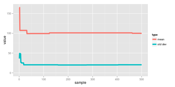
for this example let's now dive a bit deeper than just the stats object. to help understand how the sampler is converging on it's results we can also dump a trace of it's progress at the end of run_mcmc.py

import numpy
for p in ['mean', 'std_dev']:
    numpy.savetxt("%s.trace" % p, model.trace(p)[:])

plotting this we can see how quickly the sampled values converged.

two normals

let's consider a slightly more complex example.

again we have some data... 107.63, 207.43, 215.84, ... that plotted looks like this...

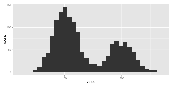
hmmm. looks like two normals this time with the one centered on 100 having a bit more data.

how could we model this one?

data = map(float, open('data', 'r').readlines())

theta = Uniform("theta", lower=0, upper=1)
bern = Bernoulli("bern", p=theta, size=len(data))

mean1 = Uniform('mean1', lower=min(data), upper=max(data))
mean2 = Uniform('mean2', lower=min(data), upper=max(data))
std_dev = Uniform('std_dev', lower=0, upper=50)

@deterministic(plot=False)
def mean(bern=bern, mean1=mean1, mean2=mean2):
    return bern * mean1 + (1 - ber) * mean2

@deterministic(plot=False)
def precision(std_dev=std_dev):
    return 1.0 / (std_dev * std_dev)

process = Normal('process', mu=mean, tau=precision, value=data, observed=True)

reviewing the code again it's mostly the same the big difference being the deterministic definition of the mean. it's now that we finally start to show off the awesome power of these non analytical approaches.

line 12 defines the mean not by one mean variable but instead as a mixture of two, mean1 and mean2. for each value we're trying to model we pick either mean1 or mean2 based on another random variable bern. bern is described by a bernoulli distribution and so is either 1 or 0, proportional to the parameter theta.

ie the definition of our mean is that when theta is high, near 1.0, we pick mean1 most of the time and when theta is low, near 0.0, we pick mean2 most of the time.

what we are solving for then is not just mean1 and mean2 but how the values are split between them (described by theta) (and note for the sake of simplicity i made the two normal differ in their means but use a shared standard deviation. depending on what you're doing this might or might not make sense)

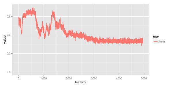
reviewing the traces we can see the converged means are 100 & 200 with std dev 20. the mix (theta) is 0.33, which all agrees with the synthetic data i generated for this example...

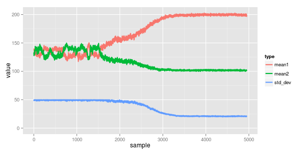
from numpy.random import normal
import random
data = [normal(100, 20) for _i in xrange(1000)]  # 2/3rds of the data
data += [normal(200, 20) for _i in xrange(500)]  # 1/3rd of the data
random.shuffle(data)

to me the awesome power of these methods is the ability in that function to pretty much write whatever i think best describes the process. too cool for school.

i also find it interesting to see how the convergence came along... the model starts in a local minima of both normals having mean a bit below 150 (the midpoint of the two actual ones) with a mixing proportion of somewhere in the ballpark of 0.5 / 0.5. around iteration 1500 it correctly splits them apart and starts to understand the mix is more like 0.3 / 0.7. finally by about iteration 2,500 it starts working on the standard deviation which in turn really helps narrow down the true means.

(thanks cam for helping me out with the formulation of this one..)

summary and further reading

these are pretty simple examples thrown together to help me learn but i think they're still illustrative of the power of these methods (even when i'm completely ignore anything to do with conjugacy)

in general i've been working through an awesome book, doing bayesian data analysis, and can't recommend it enough.

i also found blog post on using jags in r was really helpful getting me going.

all the examples listed here are on github.

next is to rewrite everything in stan and do some comparision between pymc, stan and jags. fun times!