brain of mat kelcey...

language models

language modelling is a classic problem in NLP; given a sequence of words such as "my cat likes to ..." what's the next word? this problem is related to all sorts of things, everything from autocomplete to speech to text.

the classic solution to language modelling is based on just counting. if a speech to text system is sure its heard "my cat likes to" but then can't decide if the next word if "sleep" or "beep" we can just look at relative counts; if we've observed in a large corpus how cats like to sleep more than they like to beep we can say "sleep" is more likely. (note: this would be different if it was "my roomba likes to ...")

the first approach i saw to solving this problem with neural nets is from bengio et al. "a neural probabilistic language model" (2003). this paper was a huge eye opener for me and was the first case i'd seen of using a distributed, rather than purely symbolic, representation of text. definitely "word embeddings" are all the rage these days!

bengio takes the approach of using a softmax to estimate the distribution of possible words given the two previous words. ie \( P({w}_3 | {w}_1, {w}_2) \). depending on your task though it might make more sense to instead estimate the likelihood of the triple directly ie \( P({w}_1, {w}_2, {w}_3) \).

let's work through a empirical comparison of these two on a synthetic problem. we'll call the first the softmax approach and the second the logisitic_regression approach.

a simple generating grammar.

rather than use real text data let's work on a simpler synthetic dataset with a vocab of only 6 tokens; "A", "B", "C", "D", "E" & "F". be warned: a vocab this small is so contrived that it's hard to generalise any result from it. in particular a normal english vocab in the hundreds of thousands would be soooooooo much sparser.

we'll use random walks on the following erdos renyi graph as a generating grammar. egs "phrases" include "D C", "A F A F A A", "A A", "E D C" & "E A A"

the main benefit of such a contrived small vocab is that it's feasible to analyse all 6³ = 216 trigrams. let's consider the distributions associated with a couple of specific (w1, w2) pairs.

F -> A -> ?

there are only 45 trigrams that this grammar generates and the most frequent one is FAA. FAF is also possible but the other FA? cases can never occur.

F A A  0.20   # the most frequent trigram generated
F A B  0.0    # never generated
F A C  0.0
F A D  0.0
F A E  0.0
F A F  0.14   # the 4th most frequent trigram

softmax

if we train a simple softmax based neural probabilistic language model (nplm) we see the distribution of \( P({w}_3 | {w}_1=F, {w}_2=A ) \) converge to what we expect; FAA has a likelihood of 0.66, FAF has 0.33 and the others 0.0

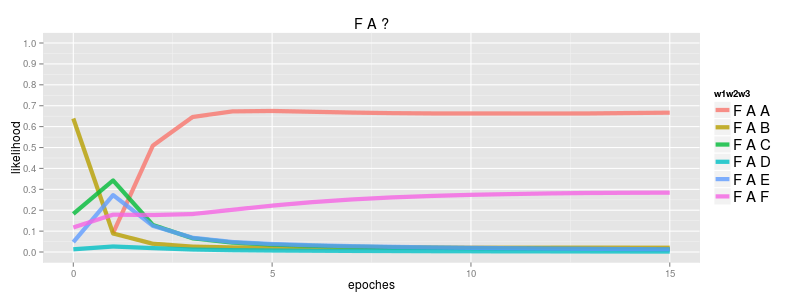
this is a good illustration of the convergence we expect to see with a softmax. each observed positive example of FAA is also an implicit negative example for FAB, FAC, FAD, FAE & FAF and as such each FAA causes the likelihood of FAA to go up while pushing the others down. since we observe FAA twice as much as FAF it gets twice the likelihood and since we never see FAB, FAC, FAD or FAE they only ever get pushed down and converge to 0.0

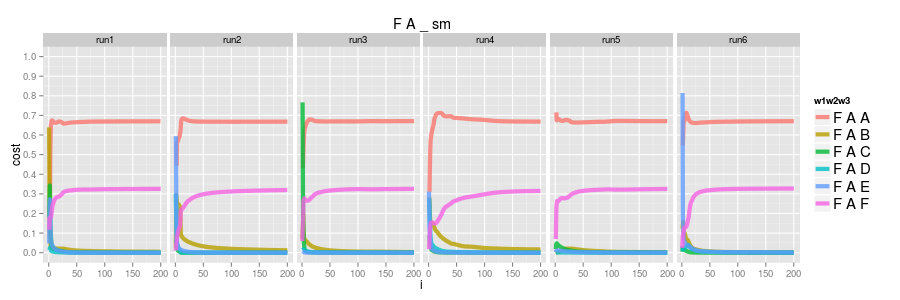
since the implementation behind this is (overly) simple we can run a couple of times to ensure things are converging consistently. here's 6 runs, from random starting parameters, and we can see each converges to the same result..

logistic regression

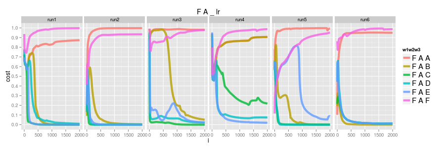
now consider the logisitic model where instead of learning the distribution of w3 given (w1, w2) we instead model the likelihood of the triple directly \( P({w}_1, {w}_2, {w}_3) \). in this case we're modelling whether a specific example is true or not, not how it relates to others, so one big con is that there are no implicit negatives like the softmax. we need explicit negative examples and for this experiment i've generated them by random sampling the trigrams that don't occur in the observed set. ( the generation of "good" negatives is a surprisingly hard problem )

if we do 6 runs again instead of learning the distribution we have FAA and FAF converging to 1.0 and the others converge to 0.0. run4 actually has FAB tending to 1.0 too but i wouldn't be surprised at all if it dropped later; these graphs in general are what i'd expect given i'm just using a fixed global learning rate (ie nothing at all special about adapative learning rate)

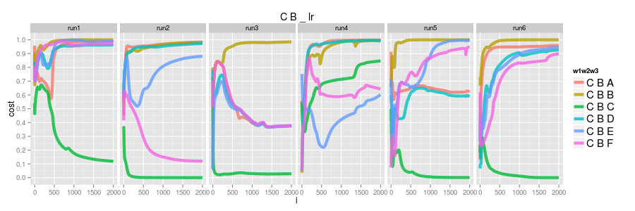
C -> B -> ?

now insteading considering the most frequent w1, w2 trigrams let's consider the least frequent.

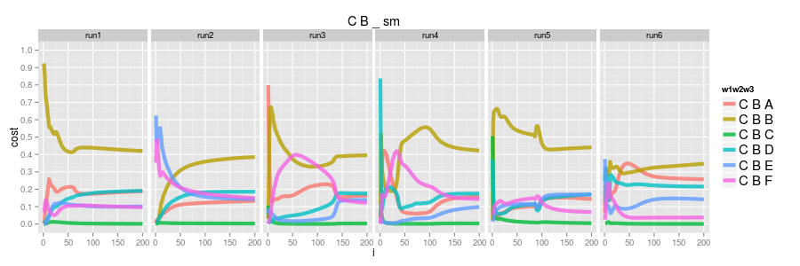
C B A  0.003
C B B  0.07   # 28th most frequent (of 45 possible trigrams)
C B C  0.0
C B D  0.003
C B E  0.002
C B F  0.001  # the least frequent trigram generated

softmax

as before the softmax learns the distribution; CBB is the most frequent, CBC has 0.0 probability and the others are roughly equal. these examples are far less frequent in the dataset so the model, quite rightly, allocates less of the models complexity to getting them right.

logisitic regression

the logisitic model as before has, generally, everything converging to 1.0 except CBC which converges to 0.0

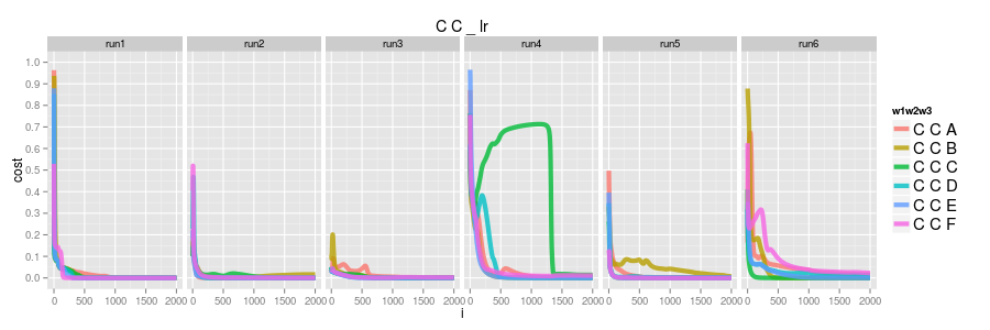
C -> C -> ?

finally consider the case of C -> C -> ?. this one is interesting since C -> C never actually occurs in the grammar.

logisitic regression

first let's consider the logistic case. CC only ever occurs in the training data as an explicit negative so we see all of them converging to 0.0 ( amusingly in run4 CCC alllllmost made it )

softmax

now consider the softmax. recall that the softmax learns by explicit positives and implicit negatives, but, since there are no cases of observed CC?, the softmax would not have seen any CC? cases.

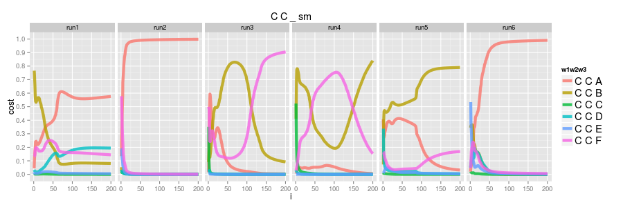
so what is going on here? the convergence is all over the place! run2 and run6 seems to suggest CCA is the only likely case whereas run3 and run4 oscillate between CCB and CCF ???

it turns out these are artifacts of the training. there was no pressure in any way to get CC? "right" so these are just the side effects of how the embeddings for tokens, particularly C in this case, are being used for the other actual observed examples. we call these hallucinations.

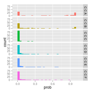
another slightly different way to view this is to run the experiment 100 times and just consider the converged state (or at least the final state after a fixed number of iterations)

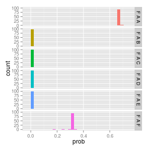
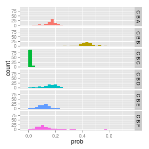
if we consider FA again we can see its low variance convergence of FAA to 0.66 and FAF to 0.33.

if we consider CB again we can see its higher variance convergence to the numbers we reviewe before; CBB ~= 0.4, CBC = 0.0 and the others around 0.15

considering CC though we see CCA and CCB have a bimodal distribution between 0.0 and 1.0 unlike any of the others. fascinating!

conclusions

this is interesting but i'm unsure how much of it is just due to an overly simple model. this implementation just uses a simple fixed global learning rate (no per weight adaptation at all), uses very simple weight initialisation and has no regularisation at all :/

all the code can be found on github