the task

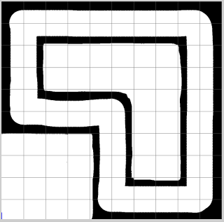
how can we train a simulated bot to drive around the following track using reinforcement learning and neural networks?

let's build something using

• the standard 2d robot simulator (STDR) as a general framework for simulating and controlling the bot ( built on top of the robot operating system (ROS) )
• tensorflow for the RL and NN side of things.

all the code can be found on github

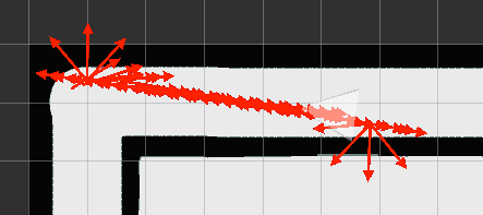
sensors

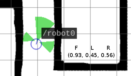
our bot has 3 sonars; one that points forward, one left and another right. like most things in ROS these sonars are made available via a simple pub/sub model. each sonar publishes to a topic and our code subscribes to these topics building a 3 tuple as shown below. the elements of the tuple are (the range forward, range left, range right).

control

the bot is controlled by three simple commands; step forward, rotate clockwise or rotate anti clockwise. for now these are distinct, i.e. while rotating the bot isn't moving forward. again this is trivial in ROS, we just publish a msg representing this movement to a topic that the bot subscribes to.

progress around track

we'll use simple forward movement as a signal the bot is doing well or not;

• choosing to move forward and hitting a wall scores the bot -1
• choosing to move forward and not hitting a wall scores the bot +1
• turning left or right scores 0

framing this as a reinforcement learning task

the reinforcement learning task is to learn a decision making process where given some state of the world an agent chooses some action with the goal of maximising some reward.

for our drivebot

• the state is based on the current range values of the sonar; this is all the bot knows
• the agent is the bot itself
• the actions are 'go forward', 'turn left' or 'turn right'
• the reward is the score based on progress

we'll call the a tuple of \( (current state, action, reward, new state) \) an event and a sequence of events an episode.

each episode will be run as 1) place the bot in a random location and 2) let it run until either a) it's not received a positive reward in 30 events (i.e. it's probably stuck) or b) we've recorded 1,000 events.

baseline

before we do anything too fancy we need to run a baseline..

if the largest sonar reading is from the forward one:
  go forward
elif the largest sonar reading is from the left one:
  turn left
else:
  turn right

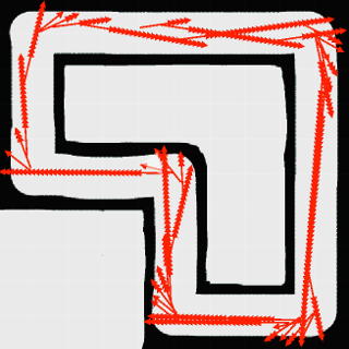
an example episode looks like this...

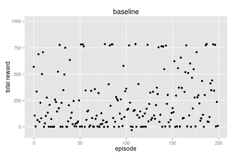
if we run for 200 episodes we can

• plot the total reward for each episode and
• build a frequency table of the (action, reward) pairs we observed during all episodes.

freq [action, reward] 47327 [F, 1] # moved forward and made progress; +1 10343 [R, 0] # turned right 8866 [L, 0] # turned left 200 [F, 0] # noise (see below) 93 [L, 1] # noise (see below) 79 [R, 1] # noise (see below) 36 [F, -1] # moved forwarded and hit wall; -1

this baseline, like all good baselines, is pretty good! we can see that ~750 is about the limit of what we expect to be able to get as a total reward over 1,000 events (recall turning gives no reward).

there are some entries that i've marked as 'noise' in the frequency table, eg [R, 1], which are cases which shouldn't be possible. these come about from how the simulation is run; stdr simulating the environment is run asynchronously to the bot so it's possible to take an action (like turning) and at the next 'tick' we've had relative movement from the action before (e.g. going straight). it's not a big deal and just the kind of thing you have to handle with async messaging (more noise).

also note that the baseline isn't perfect and it doesn't get a high score most of the time. there are two main causes of getting stuck.

• it's possible to get locked into a left, right, left, right oscillation loop when coming out of a corner.
• if the bot tries to take a corner too tightly the front sonar can have a high reading but the bot can collide with the corner. (note the "blind spot" between the front and left/right sonar cones)

q learning

our first non baseline will be based on discrete q learning. in q learning we learn a Q(uality) function which, given a state and action, returns the expected total reward until the end of the episode (if that action was taken).

\( Q(state, action) = expected reward until end of episode \)

q tables

in the case that both the set of states and the set of actions are discrete we can represent the Q function as a table.

even though our sonar readings are a continuous state (three float values) we've already been talking about a discretised version of them; the mapping to one of furthest_sonar_forward, furthest_sonar_left, furthest_sonar_right.

a q table that corresponds to the baseline policy then might look something like ...

                                     actions
state                    go_forward  turn_left  turn_right
furthest_sonar_forward          100         99          99
furthest_sonar_left              95         99          90
furthest_sonar_right             95         90          99

once we have such a table we can make optimal decisions by running \( Q(state, action) \) for all actions and choosing the highest Q value.

but how would we populate such a table in the first place?

value iteration

we'll use the idea of value iteration. recall that the Q function returns the expected total reward until the end of the episode and as such it can be defined iteratively.

given an event \( (state_1, action, reward, state_2) \) we can define \( Q(state_1, action) \) as \(reward\) + the maximum reward that's possible to get from \(state2\)

\( Q(s_1, a) = r + max_{a'} Q(s_2, a') \)

if a process is stochastic we can introduce a discount on future rewards, gamma, that reflects that immediate awards are to be weighted more than potential future rewards. (note: our simulation is totally deterministic but it's still useful to use a discount to avoid snowballing sums)

\( Q(s_1, a) = r + gamma . max_{a'} Q(s_2, a') \)

given this definition we can learn the q table by populating it randomly and then updating incrementally based on observed events.

\( Q(s_1, a) = alpha . Q(s_1, a) + (1 - alpha) . (r + gamma . max_{a'} Q(s_2, a')) \)

running this policy over 200 episodes ( \( gamma = 0.9, alpha = 0.1 \) ) from a randomly initialised table we get the following total rewards per episode.

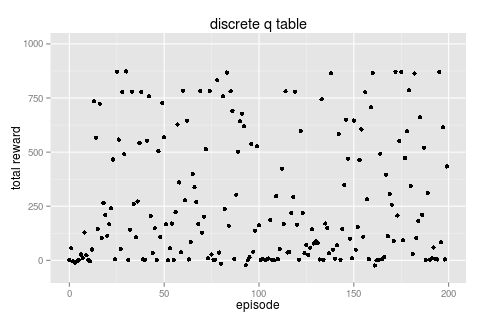
freq [action, reward] 52162 [F, 1] 10399 [R, 0] 7473 [L, 0] 1983 [R, 1] # noise 1112 [L, 1] # noise 221 [F, -1] 191 [F, 0] # noise

this looks very much like the baseline which is not surprising since the actual q table entries end up defining the same behaviour.

                                      actions
state                    go_forward  turn_left  turn_right
furthest_sonar_forward          8.3        4.5         4.3
furthest_sonar_left             2.5        2.5         5.9
furthest_sonar_right            2.5        6.1         2.4

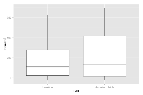
also note how quickly this policy was learnt. for the first few episodes the bot wasn't doing great but it only took ~10 episodes to converge.

comparing the baseline to this run it's maybe fractionally better, but not by a whole lot...

continuous state

using a q table meant we needed to map our continuous state space (three sonar readings) to a discrete one (furthest_sonar_forward, etc) and though this mapping seems like a good idea maybe we can learn better representations directly from the raw sonars? and what better tool to do this than a neural network! #buzzword

inference

first let's consider the decision making side of things; given a state (the three sonar readings) which action shall we take? an initial thought might be to build a network representing \( Q(s, a) \) and then run it forward once for each action and pick the max Q value. this would work but we're actually going to represent things a little differently and have the network output the Q values for all actions every time. we can simply run an arg_max over all the Q values to pick the best action.

training

how then can we train such a network? consider again our original value update equation ...

\( Q(s_1, a) = r + gamma . max_{a'} Q(s_2, a') \)

we want to use our Q network in two ways.

• for the left hand side, s1, we want to calculate the Q value for a particular action \( a \)
• for the right hand side, s2, we want to calculate the maximum Q value across all actions.

our network is already setup to do s2 well but for s1 we actually only want the Q value for one action not all of them. to pull out the one we want we can use a one hot mask followed by a sum to reduce to a single value. it may seem like a clumsy way to calculate it but having the network set up like this is worth it for the inference case and the calculation for s2 (both of which require all values)

once we have these two values it's just a matter of including the reward and discount ( \(gamma\) ) and minimising the difference between the two sides (called the temporal difference). squared loss seems to work fine for this problem.

graphically the training graph looks like the following. recall that a training example is a single event \( (state_1, action, reward, state_2) \) where in this network the action is represented by a one hot mask over all the actions.

training this network (the Q network being just a single layer MLP with 3 nodes) gives us the following results.

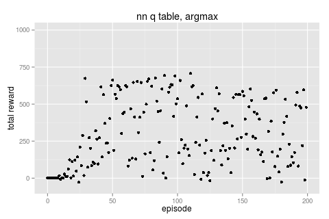
freq [action, reward] 62644 [F, 1] 36530 [R, 0] 6217 [F, -1] 3636 [R, 1] # noise

this network doesn't score as high as the discrete q table and the main reason is that it's gotten stuck in a behavioural local minima.

looking at the frequency of actions we can see this network never bothered with turning left and you can actually get a semi reasonable result if you're ok just doing 180 degree turns all the time...

even still this approach is (maybe) doing slightly better than the discrete case...

note there's nothing in the reward system that heavily punishes going backwards, you might "waste" some time turning around but the reward system is any movement not just movement forward. we'll come back to this when we address a slightly harder problem but for now this brings up a common problem in all decision making processes; the explore/exploit tradeoff.

explore / exploit

there are lots of ways of handling explore vs exploit and we'll use a simple approach that has worked well for me in the past..

given a set of Q values for actions, say, [ 6.8, 7.7, 3.9 ] instead of just picking the max, 0.8, we'll do a weighted pick by sampling from the distribution we get by normalising the values [ 0.36, 0.41, 0.21 ]

further to this we'll either squash (or stretch) the values by raising them to a power \( rho \) before normalising them.

• when \(rho\) is low, e.g. \(rho\)=0.01, values are squashed and the weighted pick is more uniform. [ 6.8, 7.7, 3.9 ] -> [ 0.3338, 0.3342, 0.3319 ] resulting in an explore like behaviour.
• when \(rho\) is high, e.g. \(rho\)=20, values are stretched and the weighted pick is more like picking the maximum. [ 6.8, 7.7, 3.9 ] -> [ 0.0768, 0.9231, 0.0000 ] resulting in an exploit like behaviour

annealing \(rho\) from a low value to a high one over training gives a smooth explore -> exploit transistion.

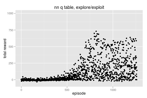
trying this with our network gives the following result.

first 200 freq [action, reward] 4598 [R, 0] 4564 [L, 0] 2862 [F, -1] 1735 [F, 1] 177 [R, 1] # noise 175 [L, 1] # noise 69 [F, 0] # noise

last 200 freq [action, reward] 45789 [F, 1] 33986 [R, 0] 4596 [F, -1] 1274 [R, 1] # noise 558 [L, 0] 36 [L, 1] # noise 1 [F, 0] # noise

this run actually kept \(rho\) low for a couple of hundred iterations before annealing it from 0.01 to 50. we can see for the first 200 episodes we have an equal mix of F, L & R (so are definitely exploring) but by the end of the run we're back to favoring just turning right again :/ let's take a closer look.

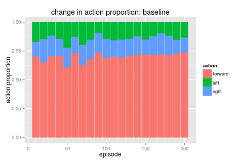
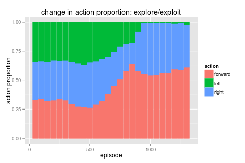
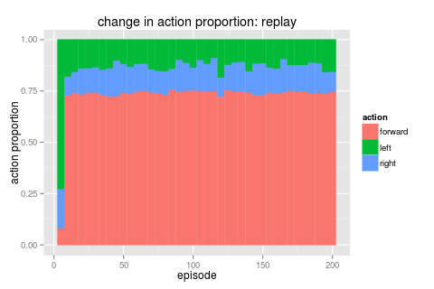
the following graphs show the proportions of actions taken over time for two runs. the first is for the baseline case and shows a pretty constant ratio of F/L/R over time. the second plot is quite different though. here we have three distinct parts; 1) a burnin period of equal F/L/R when the bot was running 100% explore 2) a period of ramping up towards exploit where we do get higher scores related to a high F amount and finally 3) where we get locked into just favoring R again.

what went wrong? and what can we do about it?

there are actually two important things happening and two clever approaches to avoiding them. you can read a lot more about these two approaches in deepmind's epic Playing Atari paper [1]

target networks

the first problem is related to the instability of training the Q network with two updates per example.

recall that each training example updates both Q(s1) and Q(s2) and it turns out it can be unstable to train both of these at the same time. a simple enough workaround is to keep a full copy of the network (called the "target network") and use it for evaluating Q(s2). we don't backpropogate updates to the target network and instead take a fresh copy from the Q(s1) network every n training steps. (it's called the "target" network since it provides a more stationary target for Q(s1) to learn against)

experience replay

the second problem is related to the order of examples we are training with.

the core sequence of an episode is \( ( state_1, action_1, reward_1, state_2, action_2, reward_2, state_3, ... ) \) which for training get's broken down to individual events i.e. \( ( state_1, action_1, reward_1, state_2 ) \) followed by \( ( state_2, action_2, reward_2, state_3 ) \) etc. as such each event's \( state_2 \) is going to be the \( state_1 \) for the next event. this type of correlation between successive examples is bad news for any iterative optimizer.

the solution is to use 'experience replay' [2] where we simly keep old events in a memory and replay them back as training examples in a random order. it's very similar to the ideas behind why we shuffle input data for any learning problem.

best result

adding these two gives the best result ...

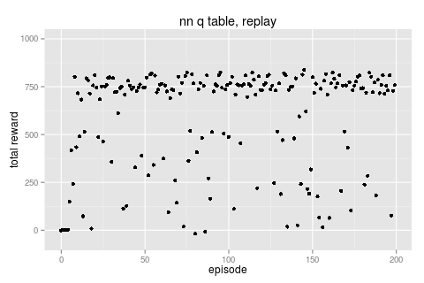
freq [action, reward] 116850 [F, 1] 18594 [R, 0] 18418 [L, 0] 2050 [L, 1] # noise 2026 [R, 1] # noise 1681 [F, -1] 1 [F, 0] # noise

this run used a bot with a high \(rho\) value (i.e. maximum exploit) that was fed 1,000 events/second randomly from the explore/exploit job. we can see a few episodes of doing poorly before converging quickly (note that this experience replay provides events a lot quicker than just normal simulation)

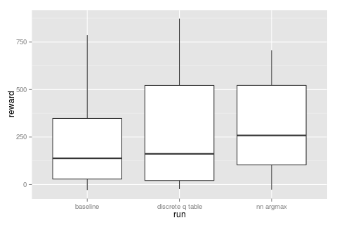
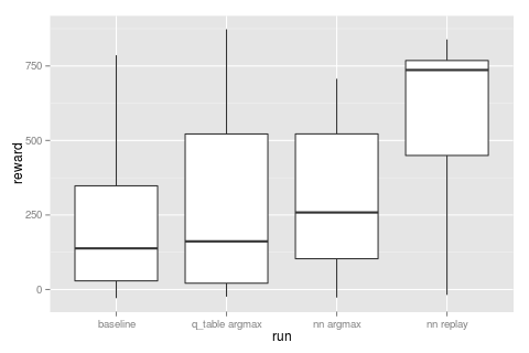
overall this approach nails it compared to the previous runs.

next steps

• a harder reward function
  • instead of a reward per movement we can give a reward only at discrete points on the track.
• continuous control
  • instead of three discrete actions we should try to learn continuous control actions ([3]) e.g. acceleration & steering.
  • will most probably require an actor/critic implementation
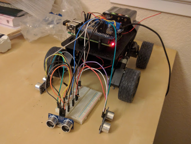
• add an adversial net [4] as a way to transfer learn between this simulated robot and the raspberry pi powered whippersnapper rover i'm building.

refs & readings

• [1] Playing Atari with Deep Reinforcement Learning (pdf)
• [2] Reinforcement Learning for Robots Using Neural Networks (pdf)
• [3] Continuous control with deep reinforcement learning (arxiv)
• [4] Domain-Adversarial Training of Neural Networks (arxiv)

follow along further with this project by reading my google+ robot0 stream

see more of what i'm generally reading on my google+ reading stream