overview

ensemble nets are a method of representing an ensemble of models as one single logical model. we use jax's vmap operation to batch over not just the inputs but additionally sets of model parameters. we propose some approaches for training ensemble nets and introduce logit dropout as a way to improve ensemble generalisation as well as provide a method of calculating model confidence.

update: though i originally developed this project using vmap, which is how things are described below, the latest version of the code is a port to use pmap so we can run on a tpu pod slice, not just one machine

background

as part of my "embedding the chickens" project i wanted to use random projection embedding networks to generate pairs of similar images for weak labelling. since this technique works really well in an ensemble i did some playing around and got the ensemble running pretty fast in jax. i wrote it up in this blog post. since doing that i've been wondering how to not just run an ensemble net forward pass but how you might train one too...

dataset & problem

for this problem we'll work with the eurosat/rgb dataset. eurosat/rgb is a 10 way classification task across 27,000 64x64 RGB images

here's a sample image from each of the ten classes...

base line model

architecture

as a baseline we'll start with a simple non ensemble network. it'll consist of a pretty vanilla convolutional stack, global spatial pooling, one dense layer and a final 10 way classification layer.

layer	shape
input	(B, 64, 64, 3)
conv2d	(B, 31, 31, 32)
conv2d	(B, 15, 15, 64)
conv2d	(B, 7, 7, 96)
conv2d	(B, 3, 3, 96)
global spatial pooling	(B, 96)
dense	(B, 96)
logits (i.e. dense with no activation)	(B, 10)

all convolutions use 3x3 kernels with a stride of 2. the conv layers and the single dense layer use a gelu activation. batch size is represented by B.

we use no batch norm, no residual connections, nothing fancy at all. we're more interested in the training than getting the absolute best value. this network is small enough that we can train it fast but it still gives reasonable results. residual connections would be trivial to add but batch norm would be a bit more tricky given how we'll build the ensemble net later.

we'll use objax to manage the model params and orchestrate the training loops.

training setup

training for the baseline will be pretty standard but let's walk through it so we can call out a couple of specific things for comparison with an ensemble net later...

( we'll use 2 classes in these diagrams for ease of reading though the eurosat problem has 10 classes. )

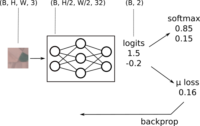
walking through left to right...

1. input is a batch of images; (B, H, W, 3)
2. the output of the first convolutional layers with stride=2 & 32 filters will be (B, H/2, W/2, 32)
3. the network output for an example two class problem are logits shaped (B, 2)
4. for prediction probabilities we apply a softmax to the logits
5. for training we use cross entropy, take the mean loss and apply backprop

we'll train on 80% of the data, do hyperparam tuning on 10% (validation set) and report final results on the remaining 10% (test set)

for hyperparam tuning we'll use ax on very short runs of 30min for all trials. for experiment tracking we'll use wandb

the hyperparams we'll tune for the baseline will be...

param	description
max_conv_size	conv layers with be sized as [32, 64, 128, 256] up to a max size of max_conv_size. i.e. a max_conv_size of 75 would imply sizes [32, 64, 75, 75]
dense_kernel_size	how many units in the dense layer before the logits
learning_rate	learning rate for optimiser

we'd usually make choices like the conv sizes being powers of 2 instead of a smooth value but i was curious about the behaviour of ax for tuning. also we didn't bother with a learning rate schedule; we just use simple early stopping (against the validation set)

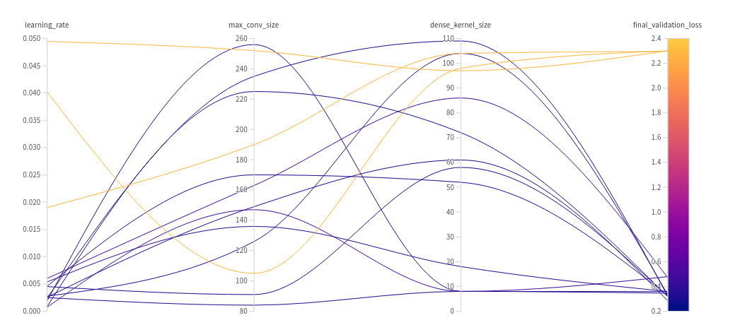
the best model of this group gets an accuracy of 0.913 on the validation set and 0.903 on the test set. ( usually not a fan of accuracy but the classes are pretty balanced so accuracy isn't a terrible thing to report. )

model	validation	test
baseline	0.913	0.903

ensemble net model

so what then is an ensemble net?

logically we can think about our models as being functions that take two things 1) the parameters of the model and 2) an input example. from these they return an output.

# pseudo code
model(params, input) -> output

we pretty much always though run a batch of B inputs at once. this can be easily represented as a leading axis on the input and allows us to make better use of accelerated hardware as well as providing some benefits regarding learning w.r.t gradient variance.

jax's vmap function makes this trivial to implement by vectorising a call to the model across a vector of inputs to return a vector of outputs.

# pseudo code
vmap(partial(model, params))(b_inputs) -> b_outputs

interestingly we can use this same functionality to batch not across independent inputs but instead batch across independent sets of M model params. this effectively means we run the M models in parallel. we'll call these M models sub models from now on.

# pseudo code
vmap(partial(model, input))(m_params) -> m_outputs

and there's no reason why we can't do both batching across both a set of inputs as well as a set of model params at the same time.

# pseudo code
vmap(partial(model)(b_inputs, m_params) -> b_m_outputs

for a lot more specifics on how i use jax's vmap to support this see my prior post on jax random embedding ensemble nets.

and did somebody say TPUs? turns out we can make ensemble nets run super fast on TPUs by simply swapping the vmap calls for pmap ones! using pmap on a TPU will have each ensemble net run in parallel! see this colab for example code running pmap on TPUs

single_input ensemble

let's walk through this in a bit more detail with an ensemble net with two sub models.

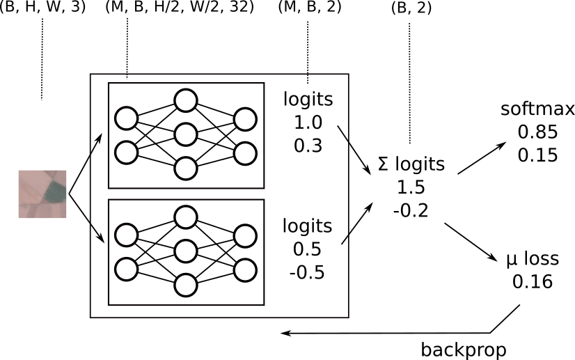
1. our input is the same as for the baseline; a batch of images (B, H, W, 3)
2. the output of the first conv layer now though has an additional M axis to represent the outputs from the M models and results in (M, B, H/2, W/2, 32)
3. this additional M axis is carried all the way through to the logits (M, B, 2)
4. at this point we have (M, B, 2) logits but we need (B, 2) to compare against (B,) labels. with logits this reduction is very simple; just sum over the M axis!
5. for prediction probabilities we again apply a softmax
6. for training we again use cross entropy to calculate the mean loss and apply backprop

this gives us a way to train the sub models to act as a single ensemble unit as well as a way to run inference on the ensemble net in a single forward pass.

we'll refer to this approach as single_input since we are starting with a single image for all sub models.

multi_input ensemble

an alternative approach to training is to provide a separate image per sub model. how would things differ if we did that?

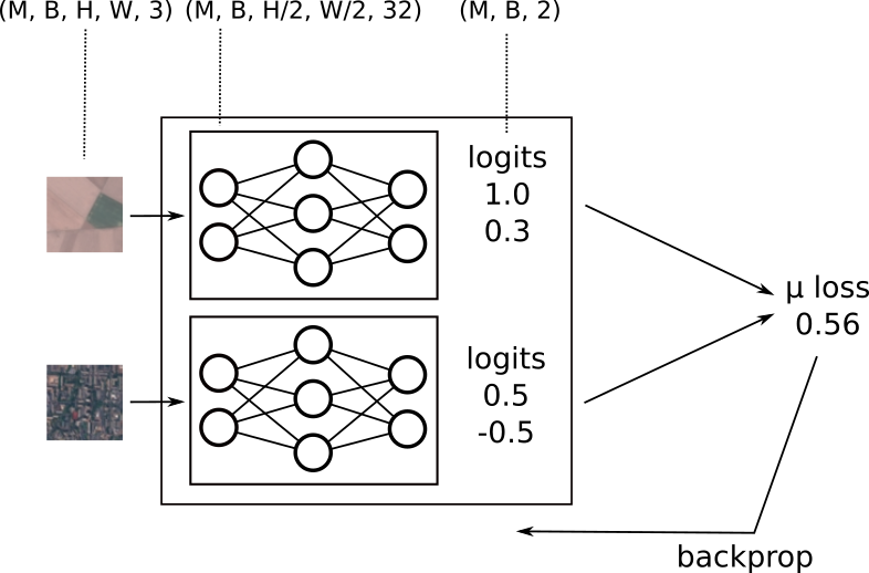
1. now our input has an additional M axis since it's a different batch per sub model. (M, B, H, W, 3)
2. the output of the first conv layers carries this M axis through (M, B, H/2, W/2, 32)
3. which is carried to the logits (M, B, 2)
4. in this case though we have M seperate labels for the M inputs so we don't have to combine the logits at all, we can just calculate the mean loss across the (M, B) training instances.

we'll call this approach multi_input. note that this way of feeding separate images only really applies to training; for inference if we want the representation of the ensemble it only really makes sense to send a batch of (B) images, not (M, B).

training the ensemble net

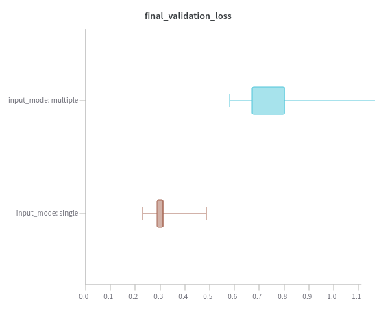
let's do some tuning as before but with a couple of additional hyper parameters that this time we'll sweep across.

we'll do each of the six combos of [(single, 2), (single, 4), (single, 8), (multi, 2), (multi, 4), (multi, 8)] and tune for 30 min for each.

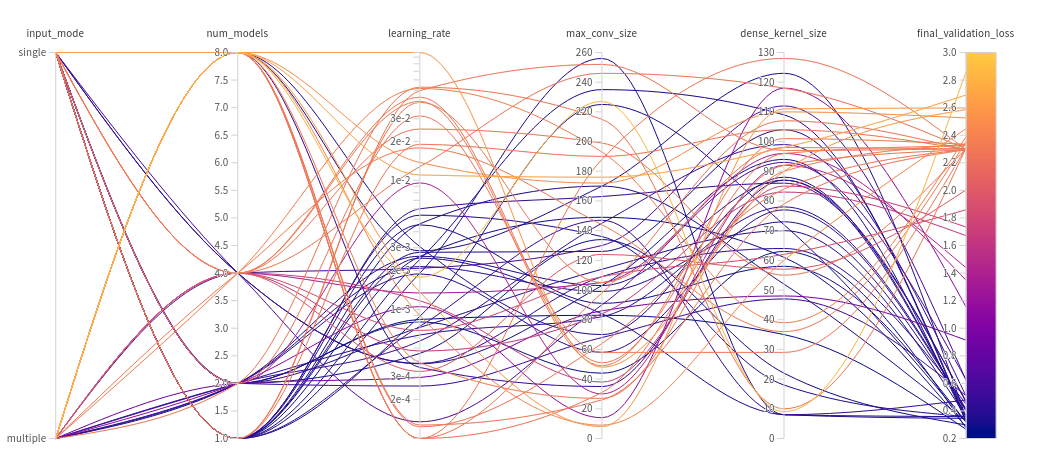
when we poke around and facet by the various params there's only one that makes a difference; single_input mode consistently does better than multi_input.

in hindsight this is not surprising i suppose since single_input mode is effectively training one network with xM parameters (with an odd summing-of-logits kind of bottleneck)

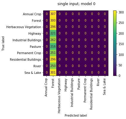
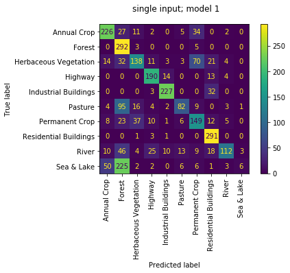
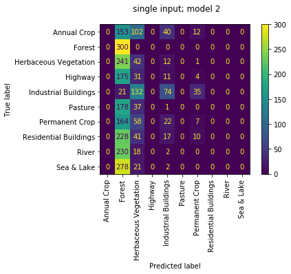
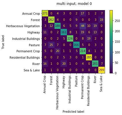
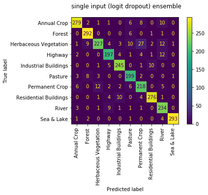
confusion matrix per sub model

single_input ensemble

when we check the best single_input 4 sub model ensemble net we get an accuracy of 0.920 against the validation set and 0.901 against the test set

model	validation	test
baseline	0.913	0.903
single_input	0.920	0.901

looking at the confusion matrix the only really thing to note is the slight confusion between 'Permanent Crop' and 'Herbaceous Vegetation' which is reasonable given the similarity in RGB.

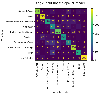
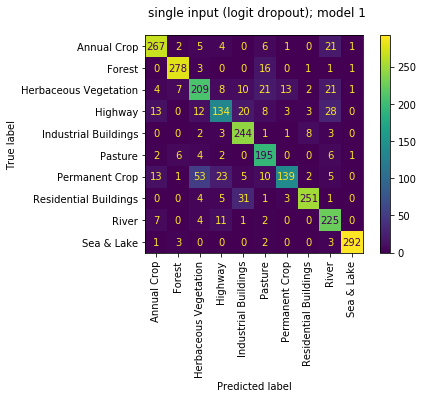
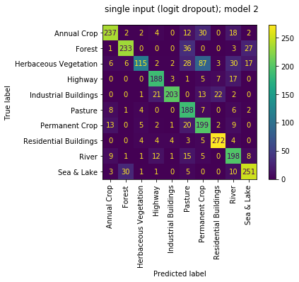
we can also review the confusion matrices of each of the 4 sub models run as individuals; i.e. not working as an ensemble. we observe the quality of each isn't great with accuracies of [0.111, 0.634, 0.157, 0.686]. again makes sense since they had been trained only to work together. that first model really loves 'Forests', but don't we all...

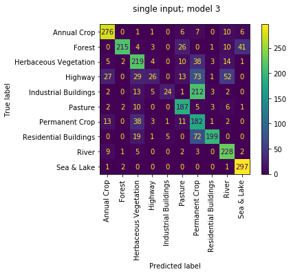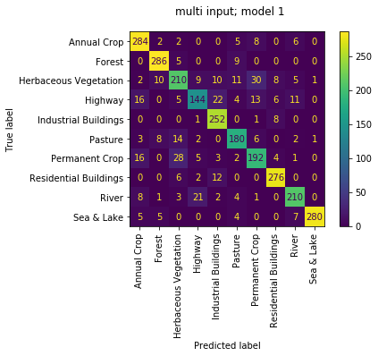
multi_input ensemble

the performance of the multi_input ensemble isn't quite as good with a validation accuracy of 0.902 and test accuracy of 0.896. the confusion matrix looks similar to the single_input mode version.

model	validation	test
baseline	0.913	0.903
single_input	0.920	0.901
multi_input	0.902	0.896

this time though the output of each of the 4 sub models individually is much stronger with accuracies of [0.842, 0.85, 0.84, 0.83, 0.86]. this makes sense since they were trained to not predict as one model. it is nice to see at least that the ensemble result is higher than any one model. and reviewing their confusion matrices they seem to specialise in different aspects with differing pairs of confused classes.

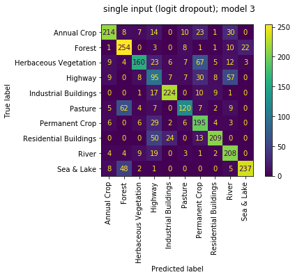
dropping logits

the main failing of the single_input approach is that the sub models are trained to always operate together; that breaks some of the core ideas of why we do ensembles in the first place. as i was thinking about this i was reminded that the core idea of dropout is quite similar; when nodes in a dense layer are running together we can drop some out to ensure other nodes don't overfit to expecting them to always behave in a particular way.

so let's do the same with the sub models of the ensemble. my first thought around this was that the most logical place would be at the logits. we can zero out the logits of a random half of the models during training and, given the ensembling is implemented by summing the logits, this effectively removes those models from the ensemble. the biggest con though is the waste of the forward pass of running those sub models in the first place. during inference we don't have to do anything in terms of masking & there's no need to do any rescaling ( that i can think of ).

so how does it do? accuracy is 0.914 against the validation set and 0.911 against the test set; the best result so far! TBH though, these numbers are pretty close anyways so maybe we were just lucky ;)

model	validation	test
baseline	0.913	0.903
single_input	0.920	0.901
multi_input	0.902	0.896
logit drop	0.914	0.911

the sub models are all now doing OK with accuracies of [0.764, 0.827, 0.772, 0.710]. though the sub models aren't as strong as the sub models of the multi_input mode, the overall performance is the best. great! seems like a nice compromise between the two!

wait! don't drop logits, drop models instead!

the main problem i had with dropping logits is that there is a wasted forward pass for half the sub models. then i realised why run the models at all? instead of dropping logits we can just choose, through advanced indexing, a random half of the models to run a forward pass through. this has the same effect of running a random half of the models at a time but only requires half the forward pass compute. this approach of dropping models is what the code currently does. (though the dropping of logits is in the git history)

using the sub models to measure confidence

ensembles also provide a clean way of measuring confidence of a prediction. if the variance of predictions across sub models is low it implies the ensemble as a whole is confident. alternatively if the variance is high it implies the ensemble is not confident.

with the ensemble model that has been trained with logit dropout we can get an idea of this variance by considering the ensemble in a hold-one-out fashion; we can obtain M different predictions from the ensemble by running it as if each of the M sub models was not present (using the same idea as the logit dropout).

consider a class that the ensemble is very good at; e.g. 'Sea & Lake'. given a batch of 8 of these images across an ensemble net with 4 sub models we get the following prediction mean and stddevs.

idx	y_pred	mean(P(class))	std(P(class))
0	Sea & Lake	0.927	0.068
1	Sea & Lake	1.000	0.000
2	Sea & Lake	1.000	0.000
3	Sea & Lake	0.999	0.001
4	Sea & Lake	0.989	0.019
5	Sea & Lake	1.000	0.000
6	Sea & Lake	1.000	0.000
7	Sea & Lake	1.000	0.000

whereas when we look at a class the model is not so sure of, e.g. 'Permanent Crop', we can see that for the lower probability cases have a higher variance across the models.

idx	y_pred	mean(P(class))	std(P(class))
0	Industrial Buildings	0.508	0.282
1	Permanent Crop	0.979	0.021
2	Permanent Crop	0.703	0.167
3	Herbaceous Vegetation	0.808	0.231
4	Permanent Crop	0.941	0.076
5	Permanent Crop	0.979	0.014
6	Permanent Crop	0.833	0.155
7	Permanent Crop	0.968	0.025

conclusions

• jax vmap provides a great way to represent an ensemble in a single ensemble net.
• we have a couple of options on how to train an ensemble net.
• the single_input approach gives a good result, but each sub model is poor by itself.
• multi_input trains each model to predict well, and the ensemble gets a bump.
• logit dropout gives a way to stop the single_input ensemble from overfitting by preventing sub models from specialising.
• variance across the sub models predictions gives a hint of prediction confidence.

TODOs

• compare the performance of single_input mode vs multi_input mode normalising for the number of effective parameters ( recall; single_input mode, without logit dropout, is basically training a single xM param large model )
• what is the effect of sharing an optimiser? would it be better to train each with seperate optimisers? can't see why; but might be missing something..

code

all on github