brain of mat kelcey...

( i've had three people recently ask me about how i was visualising gradient norms in tensorboard so, according to my three strikes rule, i now have to "automate" it by writing a blog post about it )

one really useful visualisation you can do while training a network is visualise the norms of the variables and gradients.

how are they useful? some random things that immediately come to mind include the fact that...

• diverging norms of variables might mean you haven't got enough regularisation.
• zero norm gradient means learning has somehow stopped.
• exploding gradient norms means learning is unstable and you might need to clip (hellloooo deep reinforcement learning).

let's consider a simple bounding box regression conv net (the specifics aren't important, i just grabbed this from another project, just needed something for illustration) ...

# (256, 320, 3)  input image

model = slim.conv2d(images, num_outputs=8, kernel_size=3, stride=2, weights_regularizer=l2(0.01), scope="c0")
# (128, 160, 8)

model = slim.conv2d(model, num_outputs=16, kernel_size=3, stride=2, weights_regularizer=l2(0.01), scope="c1")
# (64, 80, 16)

model = slim.conv2d(model, num_outputs=32, kernel_size=3, stride=2, weights_regularizer=l2(0.01), scope="c2")
# (32, 40, 32)

model = slim.conv2d(model, num_outputs=4, kernel_size=1, stride=1, weights_regularizer=l2(0.01), scope="c3")
# (32, 40, 4)  1x1 bottleneck to get num of params down betwee c2 & h0

model = slim.dropout(model, keep_prob=0.5, is_training=is_training)
# (5120,)  32x40x4 -> 32 is where the majority of params are so going to be most prone to overfitting.

model = slim.fully_connected(model, num_outputs=32, weights_regularizer=l2(0.01), scope="h0")
# (32,)

model = slim.fully_connected(model, num_outputs=4, activation_fn=None, scope="out")
# (4,) = bounding box (x1, y1, dx, dy)

a simple training loop using feed_dict would be something along the lines of ...

optimiser = tf.train.AdamOptimizer()
train_op = optimiser.minimize(loss=some_loss)

with tf.Session() as sess:
  while True:
    _ = sess.run(train_op, feed_dict=blah)

but if we want to get access to gradients we need to do things a little differently and call compute_gradients and apply_gradients ourselves ...

optimiser = tf.train.AdamOptimizer()
gradients = optimiser.compute_gradients(loss=some_loss)
train_op = optimiser.apply_gradients(gradients)

with tf.Session() as sess:
  while True:
    _ = sess.run(train_op, feed_dict=blah)

with access to the gradients we can inspect them and create tensorboard summaries for them ...

optimiser = tf.train.AdamOptimizer()
gradients = optimiser.compute_gradients(loss=some_loss)
l2_norm = lambda t: tf.sqrt(tf.reduce_sum(tf.pow(t, 2)))
for gradient, variable in gradients:
  tf.summary.histogram("gradients/" + variable.name, l2_norm(gradient))
  tf.summary.histogram("variables/" + variable.name, l2_norm(variable))
train_op = optimiser.apply_gradients(gradients)

with tf.Session() as sess:
  summaries_op = tf.summary.merge_all()
  summary_writer = tf.summary.FileWriter("/tmp/tb", sess.graph)
  for step in itertools.count():
    _, summary = sess.run([train_op, summaries_op], feed_dict=blah)
    summary_writer.add_summary(summary, step)

( though we may only want to run the expensive summaries_op once in awhile... )

with logging like this we get 8 histogram summaries per variable; the cross product of

• layer weights vs layer biases
• variable vs gradients
• norms vs values

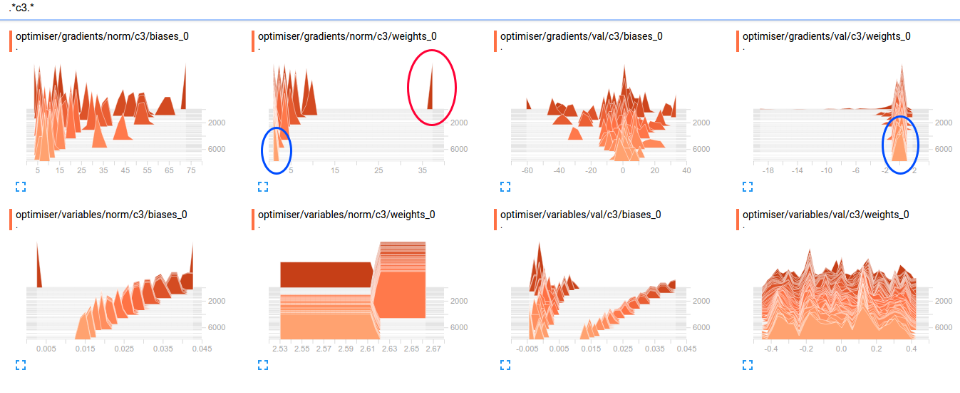
e.g. for conv layer c3 in the above model we get the summaries shown below. note: nothing terribly interesting in this example, but a couple of things

• red : very large magnitude of gradient very early in training; this is classic variable rescaling.
• blue: non zero gradients at end of training, so stuff still happening at this layer in terms of the balance of l2 regularisation vs loss. (note: no bias regularisation means it'll continue to drift)

gradient norms with ggplot

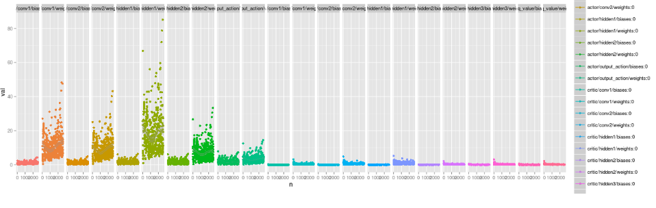
sometimes the histograms aren't enough and you need to do some more serious plotting. in these cases i hackily wrap the gradient calc in tf.Print and plot with ggplot

e.g. here's some gradient norms from an old actor / critic model (cartpole++)

related: explicit simple_value and image summaries

on a related note you can also explicitly write summaries which is sometimes easier to do than generating the summaries through the graph.

i find this especially true for image summaries where there are many pure python options for post processing with, say, PIL

e.g. explicit scalar values

summary_writer =tf.summary.FileWriter("/tmp/blah")
summary = tf.Summary(value=[
  tf.Summary.Value(tag="foo", simple_value=1.0),
  tf.Summary.Value(tag="bar", simple_value=2.0),
])
summary_writer.add_summary(summary, step)

e.g. explicit image summaries using PIL post processing

summary_values = []  # (note: could already contain simple_values like above)
for i in range(6):
  # wrap np array with PIL image and canvas
  img = Image.fromarray(some_np_array_probably_output_of_network[i]))
  canvas = ImageDraw.Draw(img)
  # draw a box in the top left
  canvas.line([0,0, 0,10, 10,10, 10,0, 0,0], fill="white")
  # write some text
  canvas.text(xy=(0,0), text="some string to add to image", fill="black")
  # serialise out to an image summary
  sio = StringIO.StringIO()
  img.save(sio, format="png")
  image = tf.Summary.Image(height=256, width=320, colorspace=3, #RGB
                           encoded_image_string=sio.getvalue())
  summary_values.append(tf.Summary.Value(tag="img/%d" % idx, image=image))
summary_writer.add_summary(tf.Summary(value=summary_values), step)