brain of mat kelcey...

neural nets on an MCU?

in my last post, wavenet on an mcu, we talked about running a cached optimised version of wavenet on an MCU at 48kHz. this time we're going to get things running on an FPGA instead!

note: this post assumes you've read that last one; it describes the model architecture, some caching tricks, and describes a waveshaping task.

neural nets on an FPGA?

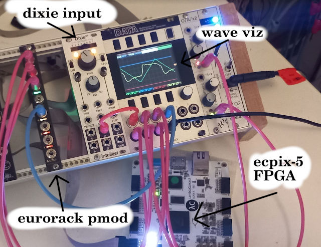
when doing some research on how to make things faster i stumbled on the eurorack-pmod project which is a piece of hardware that connects an FPGA with a eurorack setup. it includes 192kHz analog-digital-analog conversion and supports 4 channels in and out. just add an FPGA! perfect!

i'd never done anything beyond blinking LEDs with an FPGA but it can't be that hard.... right? right?!?!

well. turns out it wasn't that simple... i couldn't find any open source examples of compiling a neural net to an FPGA. the closest was HLS4ML but, if i understand it correctly, it works only with (expensive) propertiary FPGA toolchains :(

HLS4ML it did at least though put me onto qkeras which is a key component we'll talk about in a second.

( not interested in details? jump straight to the bottom for the demos )

multiple versions for training and optimised inference

recall from the last post that an important aspect of the MCU project was having multiple versions for training vs inference

• a keras version; the main version for training the weights. code
• a cmsisdsp_py version; a python prototype used to develop the caching inference & understand the cmsis api. code
• an inference firmware; the final c++ firmware for running on the MCU using cmsis-dsp for all the matrix math code

the FPGA version ended with a similar collection of variants;

• a qkeras version; main version for training quantised weights. code
• a fxpmath version; a python prototype of hand rolled fixed point inference ( reusing the caching inference from the MCU version ). code
• a verilog version; an FPGA version running first in simulation and then on eurorack pmod hardware. code

for both the MCU and FPGA versions we use a single firmware running on the daisy patch for training data collection.

let's expand on each part of the FPGA version...

qkeras

neural networks end up doing a lot of matrix multiplication. a lot.

for training it's common to work with a floating point representation since it gives the best continuous view of the loss space.

but for inference we can often reduce the precision of the weights and use integer arithmetic. we're motivated to do this since, for a lot of systems, integer math is much faster to run than full floating point math.

( and, actually, in a lot of systems we just simply might not have the ability to do floating point math at all! )

the systems we use for converting from floats during training to something simpler for inference is called quantisation and we'll look at two flavours for this project.

side note 1; fixed point arithmetic

for this project i mainly used fixed point numbers.

fixed point numbers are a simpler representation of floating point numbers with some constraints around range and precision but they allow the multiplication to be done as if it were integer multiplication. ( this is the first project i've done with fixed point math and i'm hooked, it's perfect for neural nets! )

the high level idea is you specify a total number of bits and then how many of those bits you want to use for the integer part of the number, and how many you want to use from representing the fractional part.

in this project all inputs, outputs, weights and biases are 16 bits in total with 4 bits for the integer and 12 bits for the fractional part. ( i.e. FP4.12 )

with "only" 4 bits for the integer part this means the range of values is +/- 2^4 = 8. though this might seem limiting, it's actually ok for a network, where generally activations etc are centered on zero ( especially if we add a bit of L2 regularisation along the way )

with 12 bits allocated to the fractional part we are able to describe numbers with a precision of 2^-12 = 0.00024.

here are some examples; we show the 16 bit binary number with a decimal point after the 4th bit to denote the change from the integer part to the fractional part.

bits	decimal
0010.0000 0000 0000	2^1 = 2
0101.0000 0000 0000	2^2 + 2^0 = 4 + 1 = 5
0000.0000 0000 0000	0
0000.1000 0000 0000	2^-1 = 0.5
0000.1001 0000 0000	2^-1 + 2^-4 = 0.5 + 0.0625 = 0.5625
0000.0000 0000 0001	2^-12 = 0.000244140625

the purpose of the qkeras model then is to train in full float32 but provide the ability to export the weights and biases in this configured fixed point configuration.

notes...

• using twos compliment for negative number means it's not quite +/-8 but it's close :)
• though the weights, biases and activations are in FP4.12 the multiplications and accumulations are calculated with FP8.24 ( since multiplying two FP4.12 numbers produces an FP8.24 result ). so in all the following we accumulate as FP8.24 and then "slice" the middle bits out to make it a FP4.12 number again.

side note 2; power of 2 quantisation

the options for quantisation can get pretty crazy too!

qkeras provides another scheme called power-of-two quantisation where all values are quantised to be only powers of two. i.e. depending on the fixed point config, a weight/bias can only only be one of [ +/- 1, 0, +/- 1/2, +/- 1/4, +/- 1/8, ...]

though this seems overly restrictive it has one HUGE important benefit... when a weight is a power of two then the "multiplication" of a feature by that weight can be simply done with a bit shift operation. and bit shifting is VERY fast.

and there are ways to "recover" representational power too, the best one i found being based around matrix factorisation.

if we have, say, a restricted weight matrix W of shape (8, 8) it can only contain those fixed values. but if we instead represent W as a a product of matrices, say, (8, 32). (32, 8) then we can see that, even though all the individual weights are restricted, the product of the matrices, an effective (8, 8) matrix, has many more possible values.

the pro is that the weights can take many more values, all the combos of w*w. the con though is we have to do two mat muls. depending on how much space we have for allocating the shift operations compared to the number of multiply unit we have, this tradeoff might be ok!

i messed around with this a lot and though it was interesting, and generally worked, it turned on that for the FPGA sizing ( i'm using at least ) the best result was to just use fixed point multiplication instead. :/ am guessing this is fault on my part in terms of poor verilog design and i still have some ideas to try at least...

fxpmath version

anyways, back to the models. the next model after the qkeras one is a fxpmath one.

the fxpmath version connects qkeras model fixed point export with the caching approach the inference logic that will go into the verilog design

the activation caching has two two elements that are basically the same as the MCU version; the left shift buffer for handling the first input and an activation cache for handling the activations between each convolutional layer.

the big difference comes in with the implementation of the convolution which i had to roll from scratch :/ but at least it allows for some very optimised parallelisation.

convolution 1d

consider a 1D convolution with kernel size K=4 & input / output feature depth of 16.

since we don't intend to stride this convolution at all ( that's handled implicitly by the activation caching ) we can treat this convolution as the following steps...

• 4 instance of an input by weight matrix multiplication; i.e. 4x a (1, 16) . (16, 16) matrix multiply.
• an accumulation of these K=4 results
• the adding of a bias
• applying an activation ( just relu for this project )

each of the x4 matrix multiplications are actually just a row by matrix multiplication, so can be decomposed into k=16 independent dot products ( we'll call this a row_by_matrix_multiply from now on )

and each of those dot products can be decomposed into k=16 independent multiplications followed by an accumulation.

the reason for being so explicit about what is independent, and what isn't, comes into play with the verilog version.

verilog version

verilog is a language used to "program" FPGAs and 's not at all like other languages, it's been really interesting to learn.

in the MPU version the two big concerns were

1. is there enough RAM to hold the samples and network? ( was never a problem ) and
2. does the code run fast enough to process a sample before the next comes in?

but the FPGA version is a little different. instead we more flexibility to design things based on what we want to run in parallel, vs what we want to run sequentially. for neural networks this gives lots of options for design!

side note 3; mats brutally short intro to verilog for matrix math

at a 30,000" view of verilog we have two main concerns; 1) executing code in parallel 2) executing blocks of code sequentially.

introducing verilog with a dot product

e.g. consider a dot product A.B with |A|=|B|=4

normally we'd think of this as simply something like a[0]*b[0] + a[1]*b[1] + a[2]*b[2] + a[3]*b[3] provided by a single np.dot call.

but if we're writing verilog we have to think of things in terms of hardware, and that means considering parallel vs sequential.

the simplest sequential way would be like the following psuedo code...

// WARNING PSEUDO CODE!
case(state):
  multiply_0:
    // recall; the following three statements are run _in parallel_ 
    accum <= 0                    // set accumulator to 0
    product <= a[0] * b[0]        // set intermediate product variable to a0.b0
    state <= multiply_1           // set the next state
  multiply_1:
    accum <= accum + product      // update accumulator with the product value from the last state
    product <= a[1] * b[1]        // set product variable to a0.b0
    state <= multiply_2           // set the next state
  multiply_2:
    accum <= accum + product
    product <= a[2] * b[2]
    state <= multiply_1
  multiply_3:
    accum <= accum + product
    product <= a[3] * b[3]
    state <= final_accumulate
  final_accumulate:
    accum <= accum + product
    state <= result_ready
  done:
    // final result available in `accum`
    state <= done

doing things this way does the dot product in 5 cycles...

an important aside...

an important aspect of how verilog works is to note that the statements in one of those case clauses all run in parallel. i.e. all right hand sides are evaluated and then assigned to the left hand side

e.g. the following would swap a and b

a <= b;
b <= a;

and if functionally equivalent to ...

b <= a;
a <= b;

so thinking in terms of sequential vs parallel we have the option to do more than one multiplication at any given time. this requires the hardware to be able to support 2 multiplications per clock cycle, but saves some clock cycles. not much in this case, but it add ups as |a| and |b| increase...

// WARNING PSEUDO CODE!
case(state):
  multiply_01:
    accum_0 <= 0
    accum_1 <= 0
    product_0 <= a[0] * b[0]
    product_1 <= a[1] * b[1]	
    state <= multiply_23
  multiply_23:
    accum_0 <= accum_0 + product_0
    accum_1 <= accum_1 + product_1  
    product_0 <= a[2] * b[2]
    product_1 <= a[3] * b[3]	
    state <= accumulate_0
  accumulate_0:
    accum_0 <= accum_0 + product_0
    accum_1 <= accum_1 + product_1    
    state <= accumulate_1
  accumulate_1:
    accum_0 <= accum_0 + accum_1
    state <= done
  done:
    // final result available in `accum_0`
    state <= done

or, if we want to go nuts, and, again, can support it, we can do all the elements multiplications at the same time, and then hierarchically accumulate the result into one.

// WARNING PSEUDO CODE!
case(state):
  multiply_all:
    // calculate all 4 elements of dot product in parallel; ( note: requires 4 available multiplication units )
    product_0 <= a[0] * b[0]
    product_1 <= a[1] * b[1]
    product_2 <= a[2] * b[2]
    product_3 <= a[3] * b[3]
    state <= accumulate_0
  accumulate_0:
    // add p0 and p1 at the same time as p2 and p3
    accum_0 <= product_0 + product_1
    accum_1 <= product_2 + product_3
  accumulate_1:
    // final add of the two
    accum_0 <= accum_0 + accum_1
    state <= done
  done:
    // final result available in `accum0`
    state <= done

this general idea of how much we do in a single clock cycles versus making values available in the next clock gives a lot of flexibility for a design

conv1d design in verilog

specifically for this neural net i've represented the K=4 conv 1d as

• a dot_product module code where the elements of dot products are calculated sequentially; i.e. x[0]*w[0] in the first step, x[1]*w[1] in the second, etc. so a dot product of N values takes N*M clock cycles ( where M is the number of cycles the multiple unit takes ) + some parallel accumulation.
• a row_by_matrix_multiply module code which runs the j=16 dot products required for each row_by_matrix_multiply in parallel
• and a conv1d module code that runs the K=4 row_by_matrix_multiplys are also in parallel, as well as handling the state machine for accumulating results with a bias and applying relu.

so we end up having all j=16 * K=4 = 64 dot products run in parallel, all together.

having said this, there are a number of ways to restructure this; e.g. if there were too many dot products to run in parallel for the 4 row_by_matrix_multiply we could run 2 of them in parallel, and then when they were finished, run the other 2. there are loads of trade offs between the number of multiple units available vs the time required to run them.

a slightly modified data set

in the MCU version i was only feeding in samples based on the embedding corner points, one of 4 types sampled randomly from...

input ( core wave, e0, e1 )	output
(triangle, 0, 0)	sine
(triangle, 0, 1)	ramp
(triangle, 1, 1)	zigzag
(triangle, 1, 0)	square

for the first FPGA version i did this but the model was large enough that it was quickly overfitting this and basically outputing noise for the intermediate points. as such for training of this model i changed things a bit to include interpolated data.

basically we emit corner points, say (e0=0, e1=1, sine wave) as well as interpolated points, where we pick two waves, say sine and ramp, and a random point between them and train for that point as an interpolated wave between the two ( using constant power interpolation )

though i couldn't get the MCU model to converge well with this kind of data, the larger FPGA variant has no problems.

i also messed around with a 3d input embeddings; to translate between any pairing, but it didn't add anything really so i stuck with 2d.

final model

where as the final MCU model was ...

---------------------------------------------------------------------------
 Layer (type)         Output Shape      Par#  Conv1D params
---------------------------------------------------------------------------
 input (InputLayer)   [(None, 256, 3)]  0
 c0a (Conv1D)         (None, 64, 4)     52    F=4, K=4, D=1, P=causal
 c0b (Conv1D)         (None, 64, 4)     20    F=4, K=1
 c1a (Conv1D)         (None, 16, 4)     68    F=4, K=4, D=4, P=causal
 c1b (Conv1D)         (None, 16, 4)     20    F=4, K=1
 c2a (Conv1D)         (None, 4, 4)      68    F=4, K=4, D=16, P=causal
 c2b (Conv1D)         (None, 4, 4)      20    F=4, K=1
 c3a (Conv1D)         (None, 1, 8)      136   F=8, K=4, D=64, P=causal
 c3b (Conv1D)         (None, 1, 8)      72    F=8, K=1
 y_pred (Conv1D)      (None, 1, 1)      13    F=1, K=1
---------------------------------------------------------------------------
Trainable params: 465
---------------------------------------------------------------------------

... the current FPGA version i'm running is ...

-----------------------------------------------------------------
 Layer (type)                Output Shape             Param #   
-----------------------------------------------------------------
 input_1 (InputLayer)        [(None, 64, 4)]          0                                                                         
 qconv_0 (QConv1D)           (None, 16, 16)           272                                                                        
 qrelu_0 (QActivation)       (None, 16, 16)           0                                                                          
 qconv_1 (QConv1D)           (None, 4, 16)            1040                                                                       
 qrelu_1 (QActivation)       (None, 4, 16)            0                                                                          
 qconv_2 (QConv1D)           (None, 1, 4)             260                                                                        
-----------------------------------------------------------------
Trainable params: 1,572
-----------------------------------------------------------------

it has the following differences

• have lowered the depth for the model from 4 to 3; a receptive field of 64 is enough to handle this waveshaping
• have dropped the secondary 1x1 conv and am just running 1 conv1d per layer; primarily because the code is just simpler this way
• all the internal filter sizes have been increase to 16d.

so compared to the MCU version

• it has x3 the params
• it's running at 192kHz instead of 32kHz ( so x4 faster )
• and is running at a utilisation of 30% instead of 88%

to be honest utilisation is a bit harder to compare; the trade off between compute and space is quite different with an FPGA design..

for each sample coming in at 192kHz the FPGA is running a simple state machine of 1) accept next sample 2) run the sequence of qconvs and activation caches, then 3) output the result and sit in a while-true loop until the next sample. when i say above the FPGA is running at 30% what i really should say is that it's spending 70% of the time in the post sample processing while-true loop waiting for the next sample.

looking at the device utilisation we have the following..

Info: Device utilisation:
Info: 	          TRELLIS_IO:    11/  365     3%
Info: 	                DCCA:     5/   56     8%
Info: 	              DP16KD:    24/  208    11%
Info: 	          MULT18X18D:   134/  156    85%
Info: 	             EHXPLLL:     1/    4    25%
Info: 	          TRELLIS_FF: 21081/83640    25%
Info: 	        TRELLIS_COMB: 44647/83640    53%
Info: 	        TRELLIS_RAMW:   192/10455     1%

the pieces of interest are...

• DP16KD: which is the amount of ( one type ) of RAM being used; this looks to be dominated by the activation cache, so with only 11% being used there is a lot of room for having more layers.
• MULT18X18D: is the big one, it's the max number of multiplication DSP units being used at any one time. in this model that qconv1 with in_dim = out_dim = 16. since it's already 85% if we wanted to increase the filter size much more we might be forced to not run all 16 dot products of the 16x16 row_by_matrix_multiply at once but instead, say, do 8 in parallel, then the other 8. this would incur a latency hit, but that's totally fine given we still have a lot of clock time available to do work between samples. the trouble is the code as written would end up being tricky to refactor.

currently things are setup so that the entire network has to run before the next sample comes in. this is just because it was the simplest thing to do while i'm learning verilog and it seems like the FPGA is fast enough for it. but with a neural net it doesn't have to be like that; we really just need to finish the first layer before next sample comes, not the whole network. as long as we don't mind a little bit of output latency we can run a layer per sample clock tick. doing this would actually delay the output by number-of-layer sample clock ticks, but at 192kHz that'd be fine :)

another way to run a bigger network is to continue using the same naive MULT18X18D dsp allocation but just use an intermediate layer twice; e.g. if you have a network input -> conv0 -> output you can get extra depth but running input -> conv0 -> conv0 -> output instead. you lose a bit of representation power, since the same layer needs to model two layers, but sometimes it's worth it. in this model we'd get extra depth without having to worry about more allocation, and we've got plenty of headroom to do more compute.

the po2 work in progress model

the work in progress model i've been tinkering with for the power of two quantisation is the following...

_________________________________________________________________
 Layer (type)                Output Shape              Param #  
_________________________________________________________________
 input_1 (InputLayer)        [(None, 640, 4)]          0                                                                          
 qconv_0_qb (QConv1D)        (None, 640, 8)            136       
 qrelu_0 (QActivation)       (None, 640, 8)            0         
 qconv_1_qb (QConv1D)        (None, 640, 8)            264       
 qrelu_1 (QActivation)       (None, 640, 8)            0         
 qconv_1_1a_po2 (QConv1D)    (None, 640, 16)           144       
 qconv_1_1b_po2 (QConv1D)    (None, 640, 8)            136       
 qrelu_1_1 (QActivation)     (None, 640, 8)            0         
 qconv_1_2a_po2 (QConv1D)    (None, 640, 16)           144       
 qconv_1_2b_po2 (QConv1D)    (None, 640, 8)            136       
 qrelu_1_2 (QActivation)     (None, 640, 8)            0         
 qconv_2_qb (QConv1D)        (None, 640, 4)            132       
_________________________________________________________________
Trainable params: 1,092
_________________________________________________________________

• the layers postfixed with _qb are the normal quantised bits layers which are fixed point weights and use MULT18X18D units for inference.
• the layers postfixed with _po2 have power-of-two weights and use just shift operators for inference.

the output quality is the same and it uses less MULT18X18D units but doesn't quite fit :)

Info: Device utilisation:
Info: 	          TRELLIS_IO:    11/  365     3%
Info: 	                DCCA:     5/   56     8%
Info: 	              DP16KD:    12/  208     5%
Info: 	          MULT18X18D:    70/  156    44%
Info: 	             EHXPLLL:     1/    4    25%
Info: 	          TRELLIS_FF: 37356/83640    44%
Info: 	        TRELLIS_COMB: 85053/83640   101%   close!!
Info: 	        TRELLIS_RAMW:    96/10455     0%

i spend a bunch of timing trying various combos of reuse of the modules but never had a design that would meet timing for the FPGA :/

i still feel i'm doing something wrong here, and might come back to it.

waveshaping wave examples

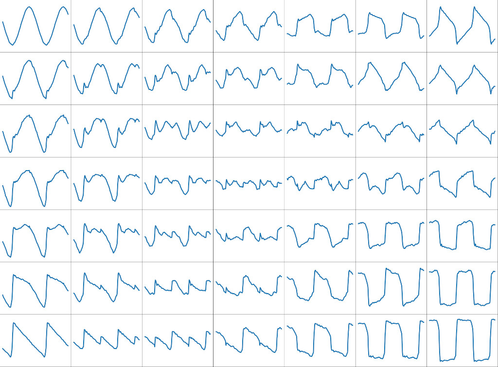waveforms generated by the model across the embedding space

the above images show the range of waveforms generated by the model across the two dimensional embedding space. of note...

• the corners represent the original logged waveshapes of ( from top left clockwise ) sine, zigzag, square and ramp. 50% of the training examples are of this type.
• the outer edges represent the examples given to the model during training, interpolated ( by constant power cross fade ) from pairs of corners. these represent the other 50% of training examples.
• the inner examples are all interpolations created by the model. note that the closer you get to the middle the further you are from a training example and the noisier the waves get...

waveshaping audio examples

lets look at some examples!

• green trace; core triangle wave being wave shaped
• blue trace; embedding x value, range -1 to 1
• red trace; embedding y value; range -1 to 1
• yellow; neural net output ( and the audio we hear )

( make sure subtitles are enabled! )

corners of the embedding space

an example of a triangle core wave as input and a manual transistion of the embedding values between the corners of the 2d space.

modulating an embedding point at audio rates

modulating the embedding x value at audio rates makes for some great timbres! the FPGA and the eurorack pmod have no problems handling this.

discontinuity glitches

since the model was trained only on a triangle wave if you give it something discontinuous, like a ramp or square, it glitches! :)

neural net techno

and if you sequence things, add an envelope to the embedding point & stick in some 909 kick & hats.... what do you have? neural net techno! doff. doff. some delay on the hats and clap, but no effects on the oscillator. ( mixed the hats too loud as well, story of my life )

TODOs

there is a lot of room to optimise for a larger network. see the issues on github

code

the code for training and verilog simulation is in this github repo

whereas the code representing this as core on the eurorack pmod is in this github repo on a branch